How to use the XLOOKUP function
XLOOKUP is a new function for Excel that offers some useful improvements over VLOOKUP and its cousin HLOOKUP (VLOOKUP looks down columns, HLOOKUP looks along rows).
Why?
In one function, XLOOKUP provides the same features that VLOOKUP and HLOOKUP offer separately, and is more powerful and easier to use. XLOOKUP also removes the need to use the INDEX/MATCH combination that allows you to work around some of VLOOKUP's shortcomings.
In this lesson, we take an in-depth look at how XLOOKUP works and provide some practical examples of how to use it.
Note: at the time of writing (September 2019), XLOOKUP is only available to users of Office365 who have joined the Office Insider Programme (you can enable this in the settings for Microsoft AutoUpdate which is installed as part of Office365). It will eventually be released more widely to Office365 users. It is not clear whether older versions of Excel will receive an update to support it.
What does XLOOKUP do?
XLOOKUP allows you to find a value in one column (or row) of data, and return a matching value from another column (or row) of data.
Here's a simple example where we want to find the price of a product where the Product ID of that product is 9823.
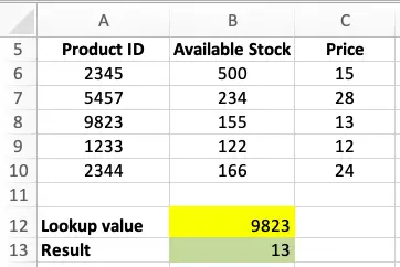
In this example, XLOOKUP looks for the value in B12 (9832) in column A (Product ID - the lookup_array). When it finds a match, it then returns the value from column C (Price - the return_array). The result is shown in B13.
The formula in B13 looks like this:
=XLOOKUP(B12,A6:A10,C6:C10)
The XLOOKUP Syntax
XLOOKUP has the following syntax. The parameters in bold are required for XLOOKUP to work. The other items extend how XLOOKUP works, and are optional:
=XLOOKUP(lookup_value, lookup_array, return_array, match_mode, search_mode)
- lookup_value is the value you are trying to find in lookup_array.
- lookup_array is a range of cells where you want to find lookup_value.
- return_array is a range of cells where the result you want is to be found
- match_mode allows you to specify how XLOOKUP searches. The default is to search for an exact match.
- search_mode allows you to change how XLOOKUP searches. The default is to start at the top of the lookup_array and work down.
We'll cover the different options for match_mode and search_mode later in the lesson. For most users, the default options will do what they need, meaning that in most cases you don't need to include them when writing a formula that uses XLOOKUP.
How is XLOOKUP different to VLOOKUP?
For most users, there are three key differences between VLOOKUP and XLOOKUP that are worth pointing out:
- VLOOKUP uses a single range of cells for both the lookup and the return. XLOOKUP requires one range for the lookup array and one for the return array. This has three key benefits:
- This allows the return array to be to the left of the lookup array, which VLOOKUP doesn't support - it can only look to the right. Without XLOOKUP, we have to use INDEX and MATCH to achieve this.
- XLOOKUP makes it easier to write a formula for looking up values in a large table where there are a lot of columns separating the lookup column and the return column, e.g. if you are looking in column A but want to return a value from column XA.
- XLOOKUP should be a lot faster for large spreadsheets with a lot of lookups and a large data table.
- VLOOKUP defaults to doing an approximate lookup.
- Most users want an exact lookup, and are confused when VLOOKUP returns a different value. However, you have to add an extra parameter to VLOOKUP if you want an exact lookup.
- XLOOKUP defaults to doing an exact lookup without requiring any extra parameters.
- When using VLOOKUP for an approximate lookup, your data must be sorted from smallest to largest in the first column for it to work correctly. Otherwise it will return a #N/A result.
- XLOOKUP does not require you to sort your data. This is a significant improvement since it is not always practical to sort your data when using VLOOKUP.
There are other differences between XLOOKUP and VLOOKUP that we'll come to later in the lesson.
XLOOKUP - Understanding match_mode
In this section we'll look more closely at how match_mode changes the way that XLOOKUP operates. This is an advanced feature that you don't need to worry about in most situations.
Earlier, we saw that match_mode is an optional parameter for XLOOKUP, and that if you omit it from your formula, XLOOKUP will default to searching for an exact match. However, there are four possible options for match_mode:
- 0 - this tells XLOOKUP to look for an exact match. As noted, you don't need to include it in your formula if this is what you want. However, if XLOOKUP doesn't find an exact match, it will return a #N/A result - which means it couldn't find a matching value.
- 1 - this tells XLOOKUP to look for an approximate match. If it can't find an exact match, XLOOKUP will look for the highest value that is less than your lookup value, and then return the result for the next higher value.
- -1 - this tells XLOOKUP to look for an approximate match. If it can't find an exact match, XLOOKUP will look for the highest value that is less than your lookup value, and then return the result for the next smaller value.
- 2 - this tells XLOOKUP to look for a wildcard value, which is used for lookups on text values. For example, if you search for Pea*, then XLOOKUP will return the first result where the first three letters of the word in the lookup_array are Pea.
Important: match_mode works for lookups with both numerical and text examples. In other words, while our examples below use the Product ID as the lookup value, they would all work if we were looking up product names instead. However, note that the Wildcard option in match_mode will only work with text values.
Let's look at examples of each option for match_mode.
Exact Match
As discussed already, XLOOKUP defaults to Exact Match if you don't specify a value for match_mode in your formula. However, you may prefer to specify it if you are also planning to specify a search_mode in your XLOOKUP formula (covered later in this lesson).
The example provided earlier in this lesson used Exact Match with this formula:
=XLOOKUP(B12,A6:A10,C6:C10)
This version of the formula specifies Exact Match as 0, and works exactly the same as the example above:
=XLOOKUP(B12,A6:A10,C6:C10,0)
Remember that Exact Match in XLOOKUP works even if your list of lookup values hasn't been sorted first. Exact Match in VLOOKUP requires that your list is sorted.
Also remember that if XLOOKUP can't find an exact match, it will return #N/A. This is not an error - it is simply Excel's way of telling us that no result could be found.
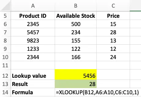
Approximate Match - Next Highest Value
The Approximate Match options require more explanation. It is useful when you need to look up values in a table where you know you won't always find an exact match. A good example might be where you are looking up a bonus percentage for a sales person, and you need to compare their sales with the different bonus thresholds.
Let's look at three examples of how Approximate Match - Next Highest Value works, using the same example we started this lesson with.
First, this example is lookup up 5456. This value does not exist in column A. XLOOKUP goes through the values from smallest to largest until it finds a value that is higher than the lookup value. In this case, that value is 5457, so XLOOKUP returns the Price for that product instead - which is 28.
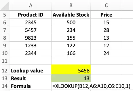
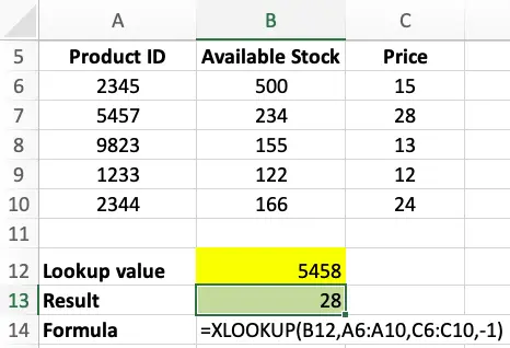
Second, this example is looking for 5458. Again, XLOOKUP finds the next highest value - 9832 - and returns the price for that product = 13.
Finally, this next example shows what happens when the lookup value - 9824 - is higher than all of the values in the list - XLOOKUP returns a #N/A result. Once again, this is not an error, simply XLOOKUP telling us it can't find a suitable match.

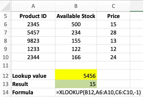
Approximate match - Next Smallest Value
This version of Approximate Match works in a similar way to the Next Highest Value, except it looks for the next smallest match in the list. Here are some examples of how it works.
First, let's use 5456 as our lookup value. This time, XLOOKUP looks for the next smallest value, which is 2345, and returns the price for that product, which is 15.
Second, this example looks for 5458. The next smallest value in the list is 5457, so the price returned is 28.
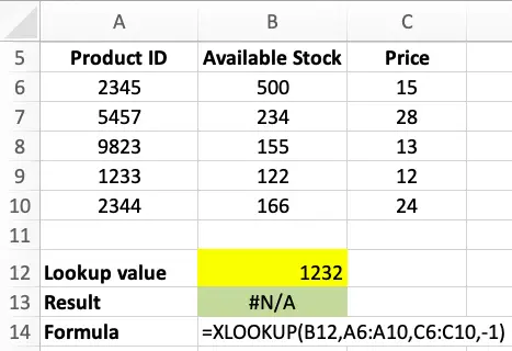
Finally, this example shows what happens when our lookup value - 1232 - is smaller than all the values in the lookup_array. As you might expect, XLOOKUP returns a #N/A result because it could not find a suitable match.
Wildcard match
Wildcard matches can be used for finding partial matches in your lookup_array.
Note that Wildcard Matches can only be used if both your lookup value and your lookup_array only contain text values. It will not work with numbers.
If your lookup value contains one of the following characters, VLOOKUP would interpret them as wildcard characters. With XLOOKUP, it will treat these characters as normal characters unless you use the Wildcard match_mode to specify that it should treat them as wildcard characters.
- * (asterisk). Used to match any number of characters.
- ? (question mark). Used to match exactly one character.
- ~ (tilde). Used when you're doing a wildcard search and you have a character that shouldn't be treated as a wildcard. For example, a Wildcard search for what is your name~? would be the same as doing an Exact Match search for what is your name?
XLOOKUP - Understanding search_mode
The final paramter in XLOOKUP is search mode. There are four possible values:
- 1 - search from the top. This is the default option - you can omit if from your formula if this is what you want.
- -1 - search from the bottom.
- 2 - search from the top in ascending order
- -2 - search from the top in descending order
Join our mailing list
Our Comment Policy.
We welcome your comments and questions about this lesson. We don't welcome spam. Our readers get a lot of value out of the comments and answers on our lessons and spam hurts that experience. Our spam filter is pretty good at stopping bots from posting spam, and our admins are quick to delete spam that does get through. We know that bots don't read messages like this, but there are people out there who manually post spam. I repeat - we delete all spam, and if we see repeated posts from a given IP address, we'll block the IP address. So don't waste your time, or ours. One other point to note - if you post a link in your comment, it will automatically be deleted.
I would like to learn how to look up a value from one worksheet to matching value in a second worksheet that has multiple rows and return the lowest date for that item.
Master Item Worksheet - Column F needs to be populated with the earliest date from Open Orders worksheet matching Item of master item worksheet (column A) to item of open orders worksheet (column B). The date to evaluate is in open orders worksheet column F - Delivery Date.