Use Conditional Formatting to highlight due dates in Excel
Excel's Conditional Formatting feature is incredibly powerful. It allows you to apply formatting to cells or ranges of cells based on criteria that you can choose. You can even use the value of other cells in the worksheet as part of your conditional formatting criteria.
This lesson uses a Project Checklist example to demonstrate how to use Conditional Formatting. The lesson is in two parts.
- First, it shows you how to apply a format to a cell containing a date where that date is in the past - this allows us to see which of the tasks in our project are overdue.
- Second, it extends the criteria for the formatting rule so that only those tasks where the due date is in the past AND the task is still open will be highlighted - at a glance, we can tell which tasks are overdue and need attention.
Note that Excel's Conditional Formatting feature includes an option to highlight dates according to a range of pre-configured conditional formatting rules. These are simple and easy to apply but the problem for our scenario is that there isn't a built-in conditional formatting rule that applies to all dates in the past - the best you can do with the built-in rules is to format cells containing dates that are in the last month. So in this lesson, we'll look at how to apply the formatting to cells containing all dates in the past, not just those in the last month.
Applying Conditional Formatting to Dates
Conditional Formatting in Excel allows you to format one or more cells based on the values in those cells. Excel offers a set of standard conditional formatting options. You can also use custom formulas to decide whether to apply a specific formatting rule to a range of cells. Using a formula as part of your conditional formatting rule is incredibly powerful, since you can incorporate cells from anywhere in your spreadsheet as part of the formula in your conditional formatting rule.
Let's start by looking at the spreadsheet that we're going to work with. This is a simple Project Checklist spreadsheet that contains the tasks that need to be completed. Each task has a status and a due date.
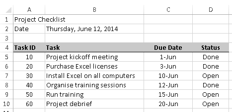
Format our cells by comparing the Due Date to the current date
In this section, we'll look at how to create a conditional formatting rule that formats the cells in the Due Date column if the task was due on a date that is in the past.
- First, select the cells you want to format:

- Next, click the Conditional Formatting button on the toolbar:

- Choose the Highlight Cells Rules option, and then select Less Than ....
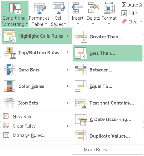
You may also notice another option in the list of Highlight Cells Rules, A Date Occurring. This is sometimes a useful option (e.g. highilight dates in the last 7 days), but it doesn't work in this scenario because it doesn't give us an option to choose all past dates. - You'll now see a dialog box like the one below in which Excel has entered a date as the LESS THAN rule (note that Excel has entered a date automatically:

- At the same time, you may notice the selected cells have been formatted as a preview of the current rule, as shown here:

- We're nearly there. As you can see, this conditional formatting rule will format all cells (i.e. all the cells we have selected) and format any cells that match our criteria with red text and light red shading. However, our rule is not quite complete - we haven't finished configuring our criteria. Remember that we want only want this rule to format cells that are in the past, i.e. before today. To do this, we'll replace the date shown with the TODAY() function which, conveniently, returns today's date.
- Here's how your completed rule should look once you enter the TODAY() function. Note that you must put the = sign at the beginning of the function so that Excel knows you're entering a formula rather than just a text value:

- Once you've done this, you can click OK and the rule will be saved and applied as shown here:

We've now completed the first part of this lesson - formatting a range of the dates in our spreadsheet so that cells containing Due Dates that are in the past will be formatted in red, as shown above. The use of the TODAY() function means that the spreadsheet will update automatically each day when you open or edit the spreadsheet.
Format our cells based on the Due Date AND the task Status
In this section, we're going to extend our conditional formatting rule so that cells with past dates will only be formatted in red if the related task is still outstanding.
To do this, we need to edit the rule we created in the previous section (rather than creating a new rule). To do this, follow these steps:
- Select the cells you want to format (i.e. the cells we formatted in the previous section)
- Click the Conditional Formatting button and choose Manage Rules. The Conditional Formatting Rules Manager will appear:

- Select the rule that needs to be edited, then click the Edit Rule ... button. As you'll see from the picture below, this looks like a version of the rule we created earlier, albeit with more information:

- At this point, we need to change our formatting rule to incorporate both of our criteria. Unfortunately, the Less Than rule we chose earlier will not longer work for us since it can't handle multiple criteria. Instead, we'll change the Rule Type to Use a formula to determine which cells to format. When you do this, the rule description will change, as shown here:

- You may also notice that I've already entered the formula we need:
- =AND(D5<>"Done",C5<TODAY()
- Here's how this formula works:
- The AND function looks at the two arguments inside the brackets and checks that both of them are true. If they are, then the AND function returns TRUE, the criteria for the rule are met and the formatting will be applied. If one or both of them are not true, then AND returns FALSE instead and the formatting is not applied. You can learn more about the AND function and its companion, the OR function, in our lesson Using logical operators and functions in Excel.
- The first argument in the AND function is D5<>"Done". This checks the Status value in column D to see if it is set to Done. If it isn't, this argument is TRUE. Note that this part of the formula uses relative references. When evaluating the status in row 5 (the first row in our table), Excel will look in D5. When evaluating row 6, Excel will look in D6, and so on. It's worth noting that I could have written the formula as D5="Open", to check if the status was set to Open. However, my projects usually have a number of status values that can be applied while a task is being worked on (Open, Pending, Waiting, Deferred) but only one status when it is done.
- The second argument in the AND function is C5<TODAY(). This is an alternative version of the rule we created in the first section - it simply looks at the value in the Due Date column to see if it is less than today's date. If it is, this argument returns TRUE.
- Once you have completed writing your formula, you can click OK to return to the Rules Manager, which now looks like this:

- Finally, you can click OK to see the results of this formula on the cells we selected. As you can see, the only row where our red formatting has been applied is row 7, where the Due Date is in the past, and the Status is Open rather than Done:

Conditional Formatting Lesson Summary
In this lesson we looked at how to create a conditional formatting rule that formats a cell containing a date if that date was prior today. We also looked at how to extend our conditional formatting rule to include criteria based on cells other than the cell that is to be formatted. In this example we only wanted to apply the formatting if the Status column was not set to Done, indicating that the task was overdue.
Conditional Formatting is a very powerful feature of Excel which can be used in a number of different ways to format cells and data automatically based on both simple and complex criteria. For another example of conditional formatting in action, check out our lesson Shade alternate rows in an Excel spreadsheet on a Mac. Even if you don't use Excel on a Mac, you'll recognise the same elements of Conditional Formatting rules, and will be able to apply the same concepts in Excel for Windows. It's also worth noting that Google Spreadsheets also support a Conditional Formatting feature; the formula I used in this example can be copied and pasted into Google's Conditional Formatting rules to achieve the same result.
Download worked examples
Join our mailing list
Our Comment Policy.
We welcome your comments and questions about this lesson. We don't welcome spam. Our readers get a lot of value out of the comments and answers on our lessons and spam hurts that experience. Our spam filter is pretty good at stopping bots from posting spam, and our admins are quick to delete spam that does get through. We know that bots don't read messages like this, but there are people out there who manually post spam. I repeat - we delete all spam, and if we see repeated posts from a given IP address, we'll block the IP address. So don't waste your time, or ours. One other point to note - if you post a link in your comment, it will automatically be deleted.
Comments on this lesson
Highlight a Cell depending of the value of another cell
Hi,
I have created a reservation list for the max. capacity of tables in a restaurant.
In the one column will be entered the number of guests, the next column calculates the amount of tables needed.
In one cell will appear the number of tables used in total with the note if tables will still be available or if the restaurant is full.
I am looking now for a formular in the conditional formating that highlights automatically the cells in the column for the needed tables if there is going to be an overbooking with the next reservation made.
To make it more understandable:
The formular of the cells for the tables needed is
=IF(D6=0,"",IF(D6<5,1,IF(D6<7,2,IF(D6<9,3,IF(D6<11,4,IF(D6<13,5,IF(D6<15,6,IF(D6<17,7))))))))
and
=IF(K6=0,"",IF(K6<5,1,IF(K6<7,2,IF(K6<9,3,IF(K6<11,4,IF(K6<13,5,IF(K6<15,6,IF(K6<17,7))))))))
For both columns the cell counting the total of tables needed
=IF(K31>24,"FULL","AVAILABLE")
Based on the total of tables needed I want the cells in the columns for the reservation of the tables to change the color as soon as the K31 shows FULL.
Thanks for your help
Formatting cells with dates
I'm attempting to write a format for our spreadsheet that tracks post-mammogram actions. I need to format the "date of exam" field to remain green for seven days and then turn red until a date is entered into the "date results sent" cell. Thanks in advance!!
Highlighting overdue dates
I am creating a spreadsheet with all staff training. Some of the Training is Mandatory and also needs to be renewed every ..12 months for example. Is there a formula that I can input that will change the date to amber if the training is coming up for renewal (e.g 4 weeks before due, and will also incorporate an additional formula that will change the date to red if overdue.
Two conditional formatting rules required
Hi Michelle
You'll need two conditional formatting rules for this, each of which applies its formatting based on a formula.
If your Due Date is in cell D6, then the formulae you need will look something like this:
- =(TODAY()-A6)<=28 (use this for the due in less than 28 days rule - it checks if the due date is less than 28 days away)
- =TODAY()>A6 (use this for the overdue rule - it checks if the due date is before today).
It doesn't matter which order these rules appear in when looking at the list of conditional formatting rules.
I hope that helps. Feel free to reply with any further questions.
Regards
David
Conditional Formatting for Expiry dates
HI there Dave
Please can you help me with a formula for columns in which I need to apply the following:
date due to expire in 60 days, then another colour if it is due to expire in 30 days, and a thrid colour if it has expired.
I have tried various ways of formatting but I cannot get 3 sets of conditions/rules to work together to change colour as appropriate.
Many thanks
Sheila
Conditional Formatting
I'm having a hard time utilizing the conditional formatting function. I am managing several pilots and I have a spreadsheet that shows when they are due certain things based upon their birth month. For example, a pilot has to take an annual exam based upon his birth month.
If he is within 30 days of his birth month or over 365 days, the cell will turn red.
If he is within 60 days but more than 30, it will turn yellow.
If he is within 90 days but less more than 60, it will be green.
All cells will have no color if he has a current date (within 90 days).
Multiple conditional rules, each with a separate formula
Hi Chuck
The key here will be to use formulas that calculate to TRUE or FALSE.
The challenge will be that you want to do things based on a comparison of the pilot's birthday and the current date.
That could be simple - your formula could be something like the following (assume the birthday is entered in C6):
=(C6-TODAY())<=30.
This will be true if the future birthday is 30 days or less from today.
Your challenge, as you've described it, is to calculate the difference between today and the first day of the month in which the pilot's birthday occurs. That's a bit harder to achieve:
First, here's a formula to return the first day of the birthday month:
=DATE(YEAR(C6),MONTH(C6),1)
This formula returns the first day of the month for the date shown in C6. This is a date value, so we can use it in a revised version of our conditional formula above:
=(DATE(YEAR(C6),MONTH(C6),1)-TODAY())<=30.
This new formula compares the first day of the month in which the pilot's birthday occurs with today. If today is within 30 days of the first day of the birthday month, this formula will return TRUE, which would trigger the conditional rule this formula is attached to.
It's slightly flawed, though, since it assumes the pilot's next birthday is happening this year, not next (e.g. what if it's December, and the birthday is in January). This formula partially addresses this scenario:
=(DATE(YEAR(C6)+(MONTH(TODAY())>=MONTH(C6),MONTH(C6),1)-TODAY())<=30.
I suspect even this formula still needs some work, e.g. what happens if TODAY() and the birthday are both in the same month, but the birthday has already happened. Should it go red? It will do with this formula.
I realize that I haven't given you a complete solution here, but hopefully it will set you on the right path. Feel free to ask more specific questions (with formula examples) here if you are still stuck.
Regards
David
Preventative Maintenance Tracker
Hi
I'm working on a spreadsheet to track all our downhole tools for their maintenance due dates.
I have a column where the current maintenance was done and another column for the due date which is 12months/365days from when maintenance was last done.
I'd like to apply a condition in which the dates under the due date column can turn Green if its within 12months and if its past 12months I'd like these cells to turn red.
Cheers
Andrew
Help
Hi,
If we would like to make a Condition Formatting formula for the cell to turn Yellow after any of the dates passed 1 week of the Reference Date and to turn Red after the date passed 2nd week (at this point, Yellow should no longer showing. Only Red).
Ex: 12th = Ref, 19th-26th = Yellow and 27th onwards = Red
Please help to advise. Thanks.
12th = Ref, 19th-26th = Yellow and 27th onwards = Red
I have a cell with a date inside of and a formula of =DATE(YEAR(H7) + 2, MONTH(H7), DAY(H7)) the question is how can i make this cell yellow at 120 days before due date and red 60 days before due date, PLEASE HELP THANK YOU
conditional Formatting help
hello. I am trying to update a number 2.5 every 30 days starting on the 1st of the month. I would also like that number to change colors from green 0-44 to yellow at 45-59 and red at 60+
so if my number starts out at 10 in 30 days starting on the 1st the number updates to 12.5 and then in 30 more days 15 etc. Any help you can provide me would be appreciated. Thank you
Please help!
I'm trying to create a heat map of tasks to see what's overdue. The logic is, is the deeadline in the past? If so is the task complete? If falseenter incomplete, if true, enter complete. The issue is I'm really struggling with future deadline dates. I've tried this formula =IF(AND(Gant!G13<>"100%",Gant!E13<TODAY()),"Overdue","Complete") which works great except fails completely with future dates as I'm asking for dates less than today.
Ideally, for future tasks was in the future it would enter the future date, if already complete it would say complete.
Many thanks for your help :)
Conditional Formatting
I am trying to format cells red, yellow, or green based on two conditions (1) past their due date and (2) percent complete. If it's past a due date and not complete it's red. If a task is due in two weeks and less than 25% it's red; due in two weeks and between 25 - 75% it's yellow; due in two weeks and >75% green. How do i do this?
Application of 2 argument formula to the rest of the excel
Hi,
So i have used the "AND" formula to apply to the single cell where it checks if the corresponding cell is either "Done" or not and then changes color.
How can i extend the application of the conditional format to do this for all the date cells to check its corresponding status?
eg. =AND($H$3<>"g",$D$3<TODAY())
Where Column D = due date
Column H = status
Do i have to create a conditional formula for every single cell separately?
Conditional Formatting - date
Thank you so much. this was quick and awesome to access and get to the answer without struggling to understand where to go. I love the visuals and explanations. Huge thanks
How to insert date auto
I need to insert date auto i.e
If i have date column D,and one column i have to insert price of an item so i need when i insert price at that time auto update the date column with current date...any one help me???
conditional formatting for a specific date
Hi,
I need to create a spreadsheet with a colour code system that will change colour based on the proximity to the due date entered in a cell. this will be a list of different dates as they are entered.
i would like them to be-
*red if it is between 0-7 days
*amber between 8-24 days
*green between 25-100 days
Is this possible? I've tried various different things with no luck :(
I
You need to figure out the right formula
Hi Emily
The question is whether you can write a set of formulas to calculate the outcomes you want.
The lesson uses this formula as an example:
=AND(D5<>"Done",C5<TODAY()
In your case, you might write something like this:
=AND((D5-TODAY())<=7,(D5-TODAY())>=0)
In this example, D5 contains the due date.
- The formula compares the due date to today's date.
- One comparison is to make sure that the due date is no more than 7 days away (<=7)
- The other comparison is to make sure that the due date is still in the future (>=0)
- The AND function means that both comparisons must be TRUE.
You would use this formula in a conditional format rule for making the colour red.
You would then create additional conditional format rules similar to this for 8-24 days (amber)and 25-100 days (green).
The key point is to remember that you can't do all of this in one single rule - you need a separate rule for each colour.
I hope that helps.
David
What formula to use if you have multiple statuses?
Thanks for this page, really useful. However, I'm a bit stuck as I need a formula which excludes formatting for when the status is either 'Completed' or 'Not required'. How would this work?
Many thanks,
Sophia
SOLVED
For anyone needing to remove the conditional formatting for two statuses rather than just one, this is the formula to use:
=AND(A1<TODAY(),OR(B1<>"Done"),OR(B1<>"Not required"))
Where A1 is the column denoting date/deadline, and B1 is the column denoting task status.
If you have three or more I think you can just keep adding OR(...) or the formula.
Conditional Formatting in Excel 2016
Hello,
I'm trying to create a suspense file of anniversary dates to show status in a separate column next to the column with dates to reflect as "Current" (if date is before today's date), however, to reflect status of "Pending" (if the date is 30 days before today's date) and future (if the date is after today's date).
Conditional formattion
HI,
I am marking progress of window installation on a project and have included in the spreadsheet some conditional formatting tasks which i'm happy with.
I want to move up to the next stage and include what i had planned and need cells highlighting according to the current date.
I have detailed what i want to do in the spreadsheet.
Thanks in advance for your help.
Dates
So I am a case manager and I complete a needs assessment when I begin workign with a client for example 6/22/2020. I need to compelte monthly notes prior to that date and would like to the column that has the Case Management needs assessment date to be highlighed 5 days before that date is on any month and then go away after that date has passed. Does this make sense. Please let me know.
Thanks,
Stacey
Conditional formatting
Hello,
I would like to create a conditional format to highlight a row (A:H)
Column A lists all days of the year as ddd-d-mmm-yy and i would like to highlight all rows that contain the 20th of each month.
thank you.
excel
I need to create a spreadsheet where i need to measure the KPI of each order placed. For Eg. order date 6th sep then it has to be shipped within 2 days (8th sep). If not then the date appears red.
How do i do that?
Conditional formatting using TODAY Function
I want to create a file that refers to the deadline on an action list so that for every action it reflects Overdue, Not due, Due in 7 days.
Conditional Formatting of training
Hello,
I have a spreadsheet that I use to track when an employee has completed their training. In the spreadsheet I enter the date it was completed. I would like the spreadsheet to highlight the specific cells when they are coming up on their renewal date. I DO NOT have a due date column. I would like the spreadsheet to take the date in the cell and add 365 days to it to determine the due date itself and then compare it to the current date to then add red highlights to the date that has past (expired), add 335 days to that date to highlight yellow for soon to expire, and all else can stay green. Is this possible?
I have multiple different training sessions so its not conducive to have a "due date" for all of these tests. Hope someone is able to help?
Conditional Formatting of training
Hello,
I have a spreadsheet that I use to track when an employee has completed their training. In the spreadsheet I enter the date it was completed. I would like the spreadsheet to highlight the specific cells when they are coming up on their renewal date. I DO NOT have a due date column. I would like the spreadsheet to take the date in the cell and add 365 days to it to determine the due date itself and then compare it to the date to then add red highlights to the date that has past (expired), add 335 days to that date to highlight yellow for soon to expire, and all else can stay green. Is this possible?
I have multiple different training sessions so its not conducive to have a "due date" for all of these tests. Hope someone is able to help?
Due Date Calculation
Hello All,
I need help in the following query:
Due Date column to dynamically change to the color's of an entire row when approaching due date. For e.g. if the task is due 10 days from due date, the row should turn orange; if the task is due 2 days from the due date, the row should turn red) Due Date column (H).
Thanks in advance
Three colour due dates
Hi there.
First of all congrats for the great job you do.
Please can you help me with a formula for columns in which I need to apply the following:
Date due to expire in 30 days, then another colour if it is due to expire in 7 days, and a thrid colour if it has expired.
Thanks a lot
Conditional Formatting
Good afternoon.
I have been watching videos and reading different "articles" on conditional formatting. What I am trying to do is set up my RFI (Request for Information) spreadsheet to track when an RFI is past due from the date it was sent, but also show the days it has been "Open".
0-10 days - Green
11-15 days - Yellow
16-20 days - Red
The kicker is I want the cell to go back to white when we enter the date we receive a response.
Any help would be greatly appreciated!
Hi,
I am looking at a spreadsheet showing all emloyees' vacations in a tracker.
I would like a red highlight to appear (perhaps in the totals column at the far right of the sheet, or on the team itself in the team column), when there is more than 40% of a team away at the SAME time.
Currently the letter "V" indicates vacation, there are rows for each employee and columns showing the dates in chronological order.
Thank you in advance to anyone who can shed some light on this!
Upa