Count the occurrences of a single character in a cell in Excel
This lesson shows you a way to calculate the number of times a single character occurs in a cell in Excel, and provides a real-life example where I needed to split a column of cells containing part numbers into individual components for each part number.
In this example, I was given a spreadsheet with a number of part number patterns. These patterns were off different lengths, and were separated into a number of individual components, each separated by a semi-colon. Part of my job involved figuring out how many components each pattern contained. Here's an example from the spreadsheet I was given:
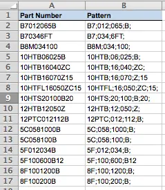
As you can see from the example above, each part number is different. In order to split each into its component parts, the first thing I need to do is write a formula to determine how many parts each pattern has.
To do this, I used the following formula:
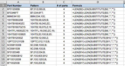
=LEN(B2)-LEN(SUBSTITUTE(B2,";",""))
Here's how my spreadsheet looked once I'd done this:
Let's break down the formula to see how it works:
=LEN(B2) |
This element of the formula counts the number of characters in B2 |
SUBSTITUTE(B2,";","") |
This element of the formula uses the SUBSTITUTE() function to replace all of the semi-colons in B2 with nothing (the third element in this formula, "", means "nothing". The result is a text value that doesn't have any semi-colons in it. We can then use the LEN() function again to find out how long the resulting text string is (see below). |
LEN(SUBSTITUTE(B2,";","")) |
By putting the LEN() function around the SUBSTITUTE() function, Excel calculates the length of the text string that is left behind if all the semi-colons are removed. By subtracting this from the first element, which was the length of the original text value, we can work out how many semi-colons were removed. |
This may seem more complicated than it needed to be. For a start, I could have simply subtracted LEN(A2) from LEN(B2). However, you won't always have all the data you need (or want) so the formula outlined in this lesson provides a more flexible way to achieve the result you're after.
Join our mailing list
Our Comment Policy.
We welcome your comments and questions about this lesson. We don't welcome spam. Our readers get a lot of value out of the comments and answers on our lessons and spam hurts that experience. Our spam filter is pretty good at stopping bots from posting spam, and our admins are quick to delete spam that does get through. We know that bots don't read messages like this, but there are people out there who manually post spam. I repeat - we delete all spam, and if we see repeated posts from a given IP address, we'll block the IP address. So don't waste your time, or ours. One other point to note - if you post a link in your comment, it will automatically be deleted.
Comments on this lesson
Thank you!
Thanks for your great solution! I used it in a slightly different context that might be of interest. I have a sheet where column A is mainly numbers in a Work Breakdown Structure style (1, 1.1, 1.1.1, etc.) and wanted a simple way to differentiate the levels without a lot of manual formatting.
Your single-formula approach works very well as a conditional format. I selected column A and applied Conditional Formatting. I selected Use a Formula to Determine Which Cells to Format and created the following formula:
=LEN(A1)-LEN(SUBSTITUTE(A1,".",""))=0 (there are 0 periods in the current cell, so it's a top-level task) make it bold
I did that a couple more times:
=LEN(A1)-LEN(SUBSTITUTE(A1,".",""))=1 (there is 1 period in the current cell) make it blue
=LEN(A1)-LEN(SUBSTITUTE(A1,".",""))=2 (means there are 2 periods in the current cell) make it red
etc. as necessary
Now when I hand the sheet off to someone, they just type in the number and the rest takes care of itself. I only wish I could indent using Conditional Formatting instead of VBA.
GREAT
Your solution worked for me... Thank You!
What an elegant solution - thanks for this.