Extract text from a cell in Excel

Sometimes it is useful (or necessary) to extract part of a cell into another cell in Excel. For example, you may have a cell that contains a combination of text and numbers, or a cell that contains two numbers separated by a delimiter such as a comma.

To do this, you can use one of the text manipulation functions available in Excel. These include LEFT() and RIGHT(). You may also need to use the LEN() function, which calculates the length of a value in a cell.

RIGHT() function syntax

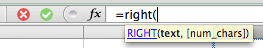
The RIGHT() function has the following syntax:

=RIGHT(text, number of characters)

The RIGHT() function works by taking the specified number of characters starting from the right end of the text value entered.

Example of the RIGHT() function in action

To use the RIGHT() function, follow these steps:

Click on a cell and enter the RIGHT() function:

Enter the two arguments for the function as shown in the following example:

The value shown in the third cell is the result of the formula, i.e. the five characters taken from a starting point of the right-most value (i.e. the last character) in the cell (A3 in this example).
- Note that in this example, the result of the RIGHT() formula, 12345, is a number and will be treated as such by Excel.
- This means that the result of the formula in this example can be used in other numerical calculations within your Excel spreadsheet.

LEFT() function syntax

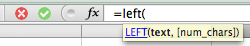
The LEFT() function has the following syntax:

=LEFT(text, number of characters)

The LEFT() function works by taking the specified number of characters starting from the left end of the text value entered.

Example of the LEFT() function in action

To use the LEFT() function, follow these steps:

Click on a cell and enter the LEFT() function:

Enter the two arguments for the function as shown in the following example:

The value shown in the third cell is the result of the formula, i.e. the 6 characters taken from a starting point of the left-most value (i.e. the first character) in the cell (A5 in this example).

MID() function syntax

The MID() function has the following syntax:

=MID(text,start_num,num_chars)

The MID function is similar to the LEFT function, except you can specify which point in the text string from which to start extracting text.

Example of the MID() function in action

In the previous example, you might enter this formula:

=MID(A5,7,3)

This would return 123 as the result; these are the three characters in the string "wilson12345", starting from the 7th character in the string.

FIND() function syntax

The FIND function is very useful in the above functions if you don't know the num_chars (i.e. the number of characters to extract) or, in the case of the MID() function, you don't know the start_num (where to start extracting text from). The FIND function can help you calculate this, which means you can write LEFT, RIGHT or MID functions that work with text strings of different lengths and components.

Examples of the FIND() function in action.

Let's work with an example where we have two text strings of different lengths, and we need to write a formula that will work with both of them.

Our example strings are wilson.12345 and tennyson.4523. We'll assume that the first value is in A1 and the second string is in A2.
Note that the number of characters and the number of digits is different in each example.
We need to convert both strings so that we are extract only the numbers from each.

The formula we need would like this:

=RIGHT(A1,LEN(A1)-FIND(".",A1))

This formula says: Take values from the right of the string, starting from the point immediately after the decimal point.

The RIGHT function says take from the right, not the left or somewhere in the middle

The num_chars value in the RIGHT function is calculated by taking the length of the value in A1 (using the LEN function) and subtracting the position of the decimal point from the length of the cell (which is determined using the FIND function).

This function will work on both of our example strings of text because the starting point is calculated using the length of the string and the position of the decimal point.

Note that this is a simple example. More complex examples might include strings that include more than one decimal point (you'd have to use the MID function as part of the solution in this case), or strings that don't have a clear delimiter (like the decimal point in this example).

There is a lot more you can do with text manipulation of cells in Excel. The LEFT(), RIGHT() and MID() functions are essential building blocks to any kind of text manipulation or text extraction in Excel.

To see more real-life examples of these functions in action, check out the comments in our lesson on converting text values to dates, where these functions are particularly useful. Here's one of my favourite examples.

Alternatively, post your own scenarios in the comments below and we'll see if we can figure out the solution for you.

Our Comment Policy.

We welcome your comments and questions about this lesson. We don't welcome spam. Our readers get a lot of value out of the comments and answers on our lessons and spam hurts that experience. Our spam filter is pretty good at stopping bots from posting spam, and our admins are quick to delete spam that does get through. We know that bots don't read messages like this, but there are people out there who manually post spam. I repeat - we delete all spam, and if we see repeated posts from a given IP address, we'll block the IP address. So don't waste your time, or ours. One other point to note - if you post a link in your comment, it will automatically be deleted.

Add a comment to this lesson

Comments on this lesson

Bringing only selected data forward

I have a job costing calculator and i only want to bring text forward to a front sheet in the workbook to summarize the selections. For example: the calculator lists several items offered, I want to bring only the items selected to a front page for a summary of the items selected to that specific job. So if there are 100 items that could be chosen, and only 5 are selected, I want to have a table that shows those 5 items only. AND the items are text not numerical value.

SO the job costing page may have : Window Removal and a cell to populate a number [number of windows to be removed] if that cell has a value greater than 0 i want the text "window removal" brought to another table for summary...I have tried IF functions and am not getting desired result...please help. Thanks

Extract number

I would like to extract the number out of column G (Description of goods) into column H (serial numbers) can you assist with a formula

Useful tips

Thanks 5 minutes were really 5 minutes and managed to extract data i wanted. Good work.

Extracting Numbers From a String

I am trying to separate the numbers from a string of text that contains numbers. The following is a sample string:
C4-14-3-6-21
I’d like to get the numbers into individual cells (except for the C4 part of the string which never changes). 14 is the year and will always be two digits. 3 will eventually become 2 digits long and then 3 and finally 4. The 6 will probably never be more than 2 digits long and the 21 can go 5 or 6 digits long. So far, I was able to create the following formulas that isolated the year (14) and the 3 (next number to the right):
=0+MID(A1,4,FIND("-",A1,4)-4)
=0+MID(A1,7,FIND("-",A1,7)-7)
It seems to work for the 14 and 3 slots. I haven’t been successful extracting the 6 and 21 (after testing different number of digits). Can you help me get these formulas right to extract all of the numbers?

Looking for similar solution

Did you ever receive a response?

LEFT

In the last exemple "=RIGHT(A1,LEN(A1)-FIND(".",A1))" how to do it to get just the names instead of the numbers? Because if you use "=LEFT(A1,LEN(A1)-FIND(".",A1))" it give all sting.

Thanks

Find it: "=LEFT(A1;FIND("/"

Find it: "=LEFT(A1;FIND("/";A1)-1)"

Extract Text from a Cell in Excel

Hi there,

I am trying to extract the set of numbers before the first "~"
My attempt using Formula=RIGHT(A1,LEN(A1)-FIND(".",A1)) returned a "0"

3932730~20~17074~S2930248~1~14~S~A-07-02-08~~1
517398~1~17074~S2930248~1~27~S~A-04-07-02
345219~1~17074~S2930248~1~5~S~A-03-01-04
239068~1~17074~S2930248~1~33~S~A-06-05-03
3935400~1~17074~S2930248~1~17~S~A-07-02-03
345219~20~17074~S2930248~1~5~S~A-03-01-04~~1
1742393~1~17074~S2930248~1~36~S~B-16-04-07

Can you please help with this? Kind regards,

Brian

Brian,

Try using =Left(A1,FIND("~",A1)-1)

Use Find/Replace

I Know I am very late, but just use replace option with text to find as "~*" and replace with null ""

Hello I'm trying to separate

Hello I'm trying to separate specific parts of text from a set of addresses. For example:
800 E DIMOND BLVD STE 127
800 E DIMOND BLVD SUITE 127
320 W 5TH AVE
3048 MOUNTAIN VIEW DR BLDG 119
2120 US HIGHWAY 92 W

On this text I would like to separate the last two parts which are "ste" and "127" to a separate column, the thing is that some addresses don't have "ste" instead they have "suite" " building", etc. Is there any way that would be possible?

Moe,

I'm sure it is possible, but I'm not the expert that could tell you how to do it. I'm sorry. I posted my original question to extract a single number from a string of numbers separated by hyphens. Try posting your question as a new string. Good luck.

Regards,

Lubo

leaving instead of extracting last octet

I am trying to get only the last octet of an ip address that is in a cell. Instead of using text to columns is there a way to leave only the last octet?

no result from Mid command

Col A B C D E F G
Invoice Status Cd State Acct Company Code Invoice Number Invoice Date Contract Number ARN
CO TX S580 65336 1/13/2014 NREC_TX_185584_CTL =MID(F2,9,6)

Using the MID formula listed under the ARN field, I am getting no result whatsoever. Excel 2007 file type .xlxs. What I want is in the ARN column G the number 185584.

minor update

dang, it didn't save my spaces betweent the column numbers. Col F has the Contract Number.

extract lot number

6006 - Silicone Tip Capsule Polisher 23gX7mm bend Lot#: 04146016 Loc.: 5
5003AF - Irrigating Cystotome 25gX16mm (5/8") formed Lot#: 12146050 Loc.: 84-86
Retrobulbar Needle 23gX1 1/2" (Atkinson Point) Lot#: 01156001

3 different rows, what I need: "Lot#: xxxxxxxx" or just the 5th digit in the lot #, in these rows it would be "6" (if you look at my attachment, Column L & M work for must but since the location [Loc] has a different number of digits, notice cell M3 cuts off some of the Lot #.

TYIA

Extracting three different parts of a cell

I need to extract three different parts in the below string of text. I need to extract flavors loved to return "Fruits, Fruits & Cream, Dessert" (it can include quotations in the text. Flavors hated "Tobacco, discovery", then Nicotine level "Low (6mg)

{"flavors_loved":["Fruits","Fruits & Cream","Dessert"],"flavors_hated":"Tobacco","discovery":"Expand Range","nicotine_level":["Low (6mg)"]}

How to extract numbers within square brackets

Hi,
I have a spreadsheet contains several thousand of records.
These records (column A) contains text strings at and numbers within a square brackets at many various lengths.
What I would like to achieve is how extract just the numbers within the square brackets of column A into a new column. Examples of records as follow;

"Bangalore Street" Beams Road [4069]
"Clifton Hill" O/B Ipswich Road FS Beaudesert Rd [10386]
"HOMEBASE" [3368]

Could someone assist me.
Thanks in advance

This is a bit messy, but it

This is a bit messy, but it works.

=mid(A1,find("[",A1)+1,find("]",A1)-find("[",A1)-1)

Thanks so much Cionn.

Thanks so much Cionn.
I've performed search & replace the open square bracket replaced with symbol then did find formular similar to yours and it works the same way as yours. Thanks for responding to my call for help. Cheers

Sorting problem

Below is a sample cell value within my spreadsheet (it's voting history- general election, primary election). I want to be able to sort using this column. The sorting would be, for example, all persons with a GE14 and a GE12 and a PE11. And various combinations like that. How could I accomplish that?

GE14GE13PE13GE12GE08GE04GE01GE00GE97

Sorting problem

GE14GE13PE13GE12GE08GE04GE01GE00GE97

More information please ...

Hi Matt

Can you be more specific about what you want to achieve? You say you want to sort, but I don't have enough information to decide where, say, someone with GE14, G13 and PE11 might be ranked compared to someone with GE14, GE13 but not PE11.

Also, can you provide a couple of additional samples, and decode the formula? For example, it looks like this is a person who voted in the General Election in 2014, 2013, 2012, 2008, 2004, 2001, 2000 and 1997, and in a Primary Election in 2013. What I can't tell is whether these are the only years in which elections were held, or if there was, say, a GE every year, but this person didn't vote in every one of them.

Thanks.

David

Hi David. Thanks for the

Hi David. Thanks for the help. The value in this column is that person's individual voting history. I'm not interested in ranking them. I only want to parcel out those people who, say, voted in GE14, GE12, and GE10. If all three of those values don't appear in this cell, then (for present sorting purposes) I'm not interested in that person. So I'm wondering what formula I would use. Some sort of if(and(search...As you've probably guessed, I'm a novice exceller. Tks for any guidance you can provide.

Finding numbers

Hi,

I am a stock markets professional and have an excel file with hundreds of records in the following sample formats:

NIFTY JUN 8500 CE
BANKNIFTY JUL 18800 PE
STAR AUG 1300 CE
INDUSINDBK JAN 900 CE
JPASSOCIAT AUG 10 PE

What I want to do is just extract the numbers out of these cells and use it in a separate formula. I would be grateful if somebody could help me with this.

Regards,

Vikas.

Extracting $ amount from a cell

Hello -

Here is an example where all I want to extract is the $4,532.50. I have several like this but not one is the same. I am just looking in that cell for the actual dollar amount and that is it. Is there a formula for that? And it can be in anywhere from $x.xx to $xxx,xxx.xx. Thanks for your assistance.

Archive Hans Wegner Table (DS) AX 2364 $4,532.50 080315 #202061,86 3520

Pulling text from the end of a string to a new column

Pulling text from the end of a string to a new column, with different length prefixes. I really need some help here :)

I need to get the size indicator of the end of the Sku into the next column
The M, XL, L and S
How can I do this because they are different lengths?

This formula is almost what I need to do.

Hello,

This formula is what I need, but I need to see another step. In my case I do have " : " and I need to grab everything as the last " : "

Example:

MY Part number: Susp IP:Torsion bars:911:1-SAW911F19

I need to grab the last part of the number just this part 1-SAW911F19

This formula almost gets me what I need =RIGHT(A1,LEN(A1)-FIND(":",A1)) but it get me everything after the first " : "

Thank you for your help.

Very percise and satisfying

Very percise and satisfying answer. Thank you so much, you are very helpful.

Same Problem here

Did you solve your problem? Mine is very similar.
rumo-log-RUMO3
bmfbovespa-BVMF3
vale-VALE5
itausa-ITSA4
banco-do-brasil-BBAS3
itau-unibanco-ITUB4
guarapes-GUAR4
braskem-BRKM5
estacio-participacoes-ESTC3
br-malls-par-BRML3
brasilagro-AGRO3
cosan-ltd-CZLT33
unicasa-UCAS3
grendene-GRND3
alupar-ALUP11
fii-cshg-jhsf-HGJH11
fii-bc-fund-BRCR11
portobello-PTBL3
mills-MILS3
cielo-CIEL3

I'm trying to get only the last caps words. This formula =RIGHT(B3;LEN(B3)-FIND("-";B3)) works great with data with only 2 words, but the rest bring me stuff that I dont need

Found it

This worked for me! =TRIM(RIGHT(SUBSTITUTE(E2,"-",REPT(" ",100)),100))

Hope it works for you too!

Great job Tiago Lemos Nascif

Also work for me

pulling text of different lengths

I am trying to pull the model of a product (text and numerical) from the beginning of each cell into another column for total product model analysis. Some models have one word, some have 3-4 words plus a number.

example:
Big River P 700c, 555, 0
Spy Hill 7.3 P 27.5, L3, 0
Glass Creek Pro Carbon Q, 29, 0

I would like to extract:
Big River
Spy Hill 7.3
Glass Creek Pro Carbon

See attached for actual data

Extracting

ip address 10.10.10.10
ip address 10.10.10.11
ip address 10.10.10.12
.
.
How can we extract only: 10.10.10.10 and 10.10.10.11 and so on?

=right(A1,11)

=right(A1,11)
If your data is in cell A1

string with unequal characters with 2 delimiters

My data is of different lengths, and the only constant is that the part I want to remove is always the last 11 characters. Alternatively, the data I want to retrieve is up to but not including the second underscore: Here is a sample:
R5510BU010_MAIN_926030_PDF
R5510BU010_MAIN_926028_PDF
R5510BU021_ALL_925732_PDF
R5510BU021_REGULAR_926026_PDF
R5510BU010_MAIN_925736_PDF
R5510BU021_REGULAR_925734_PDF
R5510BU010_MAIN_925738_PDF
R5510BU021_ALL_926024_PDF
R5510BU021_REGULAR_925468_PDF
R5510BU010_MAIN_925470_PDF
R5510BU010_MAIN_925472_PDF

What I am trying to do is retrieve everything up to but not including the second underscore. I can't use left because the fields are unequal lengths, and when I use right, it returns the stuff I'm trying to remove.

Is there a better way?

Thanks

Addendum to above question

Sorry, I forgot to add:

I tried this formula: =LEFT(G2,LEN(G2)-FIND("_",G2)) and it returned:

R5510BU010_MAIN
R5510BU010_MAIN
R5510BU021_ALL
R5510BU021_REGULAR
R5510BU010_MAIN
R5510BU021_REGULAR
R5510BU010_MAIN
R5510BU021_ALL
R5510BU021_REGULAR
R5510BU010_MAIN
R5510BU010_MAIN

This looks great, but when I copied to down to the rest of the cells I got this:

R09801_ZJDE0002_926264_PDF returned R09801_ZJDE0002_926
R09801_ZJDE0002_925803_PDF returned R09801_ZJDE0002_925
R09801_ZJDE0002_925801_PDF returned R09801_ZJDE0002_925
R09801_ZJDE0002_925805_PDF returned R09801_ZJDE0002_925
R09801_ZJDE0002_925807_PDF returned R09801_ZJDE0002_925
R09801_ZJDE0002_925809_PDF returned R09801_ZJDE0002_925
R09801_ZJDE0002_925811_PDF returned R09801_ZJDE0002_925
R09801_ZJDE0002_926290_PDF returned R09801_ZJDE0002_926

Why did it seem to understand in the first selection but not the second?

Thanks

Ease of access to specific issues in 5 minute lessons

Thank you very much for putting up 5 minute lessons. They work better than excel help menu and the explanations are far more comprehensive & useful. I use 5 minute lesson as my excel help menu.

Extract text from a cell

I have a situation where I need to extract some or all of the DATA in a cell.
I am an options trader and at the end of the day i would like to know the underlying stock symbol for the option which will help easily filter and sort the trades.

stock symbols normally range between 1 and 4 letters

GDX
GDX 160708P28
GDX 160708P28
BBRY 160916C9
SLV 160805C19.5
SLV

=LEFT(B11,FIND(" ",B11))
This works fine for the option chain, but if its just the stock"SLV" it returns an error

The values im looking for are listed below
GDX
GDX
GDX
BBRY
SLV
SLV

Thanks for your help

Extracting Multiple info from a string of text

The below contains info found in a cell separated by commas. I'd to separate each of the info grouped by commas and put into different cells. At the moment I can only extract only the first set "PKL70080P" using =LEFT(A65,FIND(",",A65)-1). The rest I'm not sure how to do that.

PKL70080P,"Tbitha 318* x .02 LB OPT",TPLin,5/12/2011,19,81,96,82,91,81,85,98,94,95,92,98,80,N/A,""

Thanks!

is it possible to get selected text from a row

example
asdfasfaffasf want to select asf

Extracting 'Sub ID'

I am trying to extract a 32 alphanumeric subscription ID out of the Forecast Comments column. Forecast comments are essentially notes exported from our CRM system. The majority of the sales reps have "Sub ID[space]" prior to the IS, so I tried =RIGHT(J2,LEN(J2)-FIND("Sub ID ",J2)) but I got an error. Also I don't want all the notes that are in the cell AFTER the Sub ID.

Extracting 'Sub ID'

i was lost in hope and faith

i was lost in hope and faith when i was unable to get into my account that i save all my document and file ,but thanks to cyberhelp company who help me get into my account and get everything back for me with no stress just give them some info and everything is done within 5hours really amazing to work with them ,thats why im so proud to recommend they to people to use them and they will never disappoint you ,,contact them on ( cyberhelp027 @ ...gmail .com ) and you thanks me later
or text them on +160 64413481 or What Sapp +1 7863616429

Extracting Data from one cell to copy in another

Hi,
I am trying to find a way of extracting only part of a cells contents if it contains certain characteristics. So in cell C2 I have a long bank narrative which may contain a policy number. They number always begin with the same 2 letters for example AB followed by 7 numbers.

How can I get excel to check C2 and if it contains anything which begins AB followed by 7 numbers it will copy the policy number to cell G2? The policy number could be anywhere in the text so it needs to be able to go through the whole cell content.

Thanks for any help you can give

Extracting Data from one cell to copy in another

Thanks for any help you can give

You are here

Search form

Extract text from a cell in Excel

RIGHT() function syntax

Example of the RIGHT() function in action

LEFT() function syntax

Example of the LEFT() function in action

MID() function syntax

Example of the MID() function in action

FIND() function syntax

Examples of the FIND() function in action.

Want to learn more? Try these lessons:

Our Comment Policy.

Comments on this lesson

Add comment

Plain text

Search

Additional Info

Similar lessons

Join our mailing list