Use COUNTIFS to count cells that match multiple criteria

The COUNTIFS function in Excel counts the number of cells in a range that match a set of multiple criteria. COUNTIFS extends the COUNTIF function which only allows one criteria. It is similar to SUMIFS, which will find the sum of all cells that match a set of multiple criteria.

COUNTIFS function syntax

The COUNTIFS function has the following syntax:

=COUNTIFS(criteria_range1,criteria1, criteria_range2,criteria2,....)

• criteria_range1 is the first range of cells
• criteria1 is the criteria should be matched against criteria_range1
• Similarly, criteria_range2 is the second range of cells that should be matched against criteria2.

There are several things you need to remember when using the COUNTIFS function in a formula:

• You can use up to XX criteria_range and criteria pairs in a single COUNTIFS function.
• Whether you have two or twenty criteria ranges, each one MUST be the same shape.

It's important to note that the COUNTIFS function takes all of the criteria_range/criteria pairs and counts only those instances where all of the pairs are true. This is best demonstrated with an example.

Scenario One - COUNTIFS with one criterion

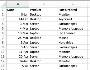
Let's say we have a list of recent computer hardware purchases as shown here:

Suppose we want to count how many times Desktop appears in the Product column. This can be done with a COUNTIF function - we don't need to use COUNTIFS at this point. Here's the formula to do this:

=COUNTIF(B2:B13,"Desktop")

Here's how that might look in our spreadsheet:

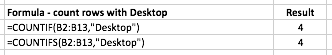
Notice that although we don't need to use COUNTIFS in this scenario, COUNTIFS will return the same result.

Also note that it is possible to use any rectangular criteria range. Our example above uses a criteria range that is 1 column wide and 12 rows deep (B2:B13).

It would also work if we used a criteria range that was, say, 2 columns wide and 12 rows deep, or even 12 columns wide and 1 row deep. COUNTIFS will simply count all of the cells in the range you specify that contain the criteria you specify.

Scenario 2 - COUNTIFS with two criteria in different criteria ranges

Once you understand how to use COUNTIFS with one critera_range and criteria, it becomes easy to extend it to two or more criteria_range/criteria combinations.

For example, let's count the number of times the combination of Desktop and Monitor appear in our spreadsheet:

=COUNTIFS(B2:B13,"Desktop",C2:C13,"Monitor")

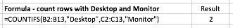
As you can see, this formula has returned the correct number of rows where both criteria are matched in their respective columns.

It's worth repeating one of the rules of COUNTIFS here - the two criteria ranges must be the same shape and size or your formula won't work, and will return a #VALUE error. Here's an example where the second criteria range is smaller than the first:

=COUNTIFS(B2:B13,"Desktop",C2:C12,"Monitor")

Scenario 3 - COUNTIFS with two criteria in the same criteria range

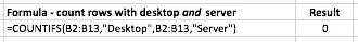
Another common scenario is to use the same criteria with more than one criteria_range. For example, suppose we want to count the number of times either Desktop or Server appear in the Product column. You might try this formula using COUNTIFS:

=COUNTIFS(B2:B13,"Desktop",B2:B13,"Server")

Unfortunately, this formula will return a value of 0, as shown here:

This is a common mistake that even experienced Excel users make when using COUNTIFS (and its counterpart, SUMIFS which you can learn about here).

The problem is that COUNTIFS looks in our criteria_range, B2:B13 and tries to count cells that contain both Desktop and Server. Remember that we wanted to count cells that contain either Desktop or Server. Of course, there are no cells in our range that contain both Desktop and Server, so the result is 0.

Ironically, the best way to find the answer in this scenario is so simple that it is often overlooked - just use two COUNTIF functions in your formula, rather than once COUNTIFS function, like this:

=COUNTIFS(B2:B13,"Desktop")+COUNTIF(B2:B13,"Server")

This yields the correct result, as shown here:

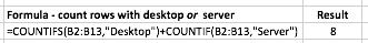
In other words, we simply count all the rows that contain Desktop, and add those to the tally of rows that contain Server.

Summary

The COUNTIFS function allows you to count the number of times