Use SUMIFS to sum cells that match multiple criteria in Excel
The SUMIFS function in Excel allows you to sum the values in a range of cells that meet multiple criteria. For example, you might use the SUMIFS function in a sales spreadsheet to to add up the value of sales of a specified product by a given sales person (e.g. the value of all sales of a microwave oven made by John). This lesson shows you how to use SUMIFS in your own spreadsheets.
Note that SUMIFS was introduced in Excel 2007. This lesson therefore only applies to Excel 2007, 2010, 2011 and 2013.
Also, you'll find a number of examples in the comments at the end of the lessons where people have been trying to use SUMIFS when a Pivot Table is a better solution. If you can't find what you want here, try our lessons on Pivot Tables instead (opens in a new tab).
Using SUMIFS - an example
Consider the following table that contains sales data:
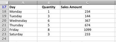
Imagine you want to add up the sales amounts that are greater than $500, and where the quantity sold was 3 or more. You could solve the problem by creating an additional column and use the IF function to evaluate the sales amount and the sales quantity and calculate whether or not to include that sales amount in the total, but that would be somewhat long-winded AND would mean you have to have another column in the table. But the SUMIFS function means you don't have to.
The SUMIFS() function syntax
The SUMIFS() function has the following syntax:
=SUMIFS(sum_range, criteria_range1, criteria1, criteria_range2, criteria2,....)
The function arguments are as follows:
- sum_range is the range of cells to be added up
- criteria_range1 is the first range of cells that are to be checked for a criteria match
- criteria1 is the criteria against which criteria_range1 is to be checked.
- criteria_range2 is the second range of cells that are to be checked for a criteria match
- criteria2 is the criteria against which criteria_range2 is to be checked.
You must have at least one criteria range and criteria. However, if you only have one criteria range, then you may as well use the SUMIF() function instead (it works in almost exactly the same way as the SUMIFS function).
SUMIFS lets you have up to 127 different sets of criteria_range and criteria. Note that the shape of each criteria_range must be the same as the shape of the sum_range. This isn't necessary with the SUMIF function.
The SUMIFS() function in action
Let's use the SUMIFS function to solve the scenario introduced at the start of this lesson.
- The table above now looks like this (I've included the SUM function so you can see the overall sales total for the table:
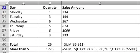
- As you'll see, B41 is showing the total sales, but only for those days where the quantity sold was greater than 3 (criteria1) and the sales amount was greater than $500 (criteria2). The two rows that meet both of these criteria in the table above are Thursday and Friday. The SUMIFS formula I used to perform this calculation is shown in cell C41 so you can see how it works.
- Remember that, as with the SUMIF function, when you're using a criteria such as "greater than", you need to use quotation marks around the criteria, i.e. ">3" and ">500".
- The same applies if you wanted to use a text criteria, such as the day of the week. An example of a text criteria might be "Thursday" if you only wanted sales made on Thursday (useful if you have a spreadsheet like this that spans several weeks).
I've included a downloadable copy of the spreadsheet above, which also includes the SUMIF examples based on the same sales table. You can use this to try out different variations on the example above. Try changing the values in the Quantity and the Sales Amount columns, and check that the formula works correctly. Then, as a stretch, try adding a third criteria range to the formula so that it only adds sales for Thursday.
Did this lesson help you understand the SUMIFS() function? Do you have an alternative scenario where you've used the SUMIFS function? Tell us about it by writing a comment below.
Our Comment Policy.
We welcome your comments and questions about this lesson. We don't welcome spam. Our readers get a lot of value out of the comments and answers on our lessons and spam hurts that experience. Our spam filter is pretty good at stopping bots from posting spam, and our admins are quick to delete spam that does get through. We know that bots don't read messages like this, but there are people out there who manually post spam. I repeat - we delete all spam, and if we see repeated posts from a given IP address, we'll block the IP address. So don't waste your time, or ours. One other point to note - if you post a link in your comment, it will automatically be deleted.
Comments on this lesson
I'd recommend you solve this using a PivotTable
You could solve this problem using SUMIF and SUMIFS, but I would recommend you use a PivotTable instead. You can learn how to use a PivotTable in this lesson. It's a lot more flexible and powerful and will do exactly what you need.
Column A=Sales Rep, Column
Column A=Sales Rep, Column B=Items, Column C=Sold Qty
I need individual record (each Sales Rep, each item ,total sold qty)
Clear and concise
Great tutorial on the use of SUMIFS . Excel is really a powerful tool and it is very helpful when one can get what they need online in the way of help. Most books that cover these topics (yes , there are still books) go into too much over the top things and don't get into the real meat of the subject - like this does, covering what I need to know ! Thank you,
excel function sto solve
Can any one please help me to use the similar formula in excel to find out
the sum the Row 3 IF row 1 is equal to "SecSch" AND row 2 is equal to "Current"
Say in excel Row 1 (contains a list of "Sec", "Pry", "RCs"), Row 2 (contains "Current" and "Capital"), and Row 3 (contains list of budget figures 135.45)
Thank you in advance
I have a column with with
I have a column with with categories and next to that are their numbers/amounts. I want to add/sum certain categories together? I have the categories identified by text ...thanks
The SUMIF function should do this for you
Hi E Dot
Sounds like you need the ordinary SUMIF function rather than the SUMIFS function. This will allow you to add up numbers that match the categories you choose. If you need to add up more than one category in a single formula, simply put multiple SUMIF functions together in the same formula. In this scenario each SUMIF function would add up all the values for one category.
Check out the SUMIF lesson here.
Regards
David
SUMIFS with multiple criteria
I beleive I understand the material, but cannot undertsand why this produces a #VALUE! error.
=SUMIFS($E$2:$E$51,$F$2:$F$51,$D81,$G$74:$G$84,$E$74)
Different sized ranges are the reason
Hi Tom
I think your problem is that the first sum range and the second are different sizes. If you change $G$74:$G$84 to $G$2:$G$51 then the formula no longer generates an error.
Given your example, I would create a formula that uses the SUMIF function twice rather than trying to use SUMIFS, e.g.
=SUMIF($E$2:$E$51,$F$2:$F$51,$D81)+SUMIF($G$74:$G$84,$E$74)
Regards
David
SUMIFS with multiple criteria
Hi David,
Thank you very much for the reply. I didn't know about using two SUMIFs.
I really appreciate your help. I'm pretty good at using arrays to explore massive amounts of data at Intel, but really ignorant of the Excel syntax to do other things.
If you have the time and interest, I try to explain better. If you don't, Thanks again.
I'm not sure if were able to look at the file and see what/where the ranges are.The error is gone, but I'm not getting the correct answer. (I didn't explain what I was trying to do, so it wasn't very clear.) After two hours of trial and error, I was crabby and desparate.
I'm trying to sum the amounts in col E by month (Col F) and by catagory 1 or 2 (Col G). Col E is month # reference and D81
is the target Category number. I'm sure there are better ways to do it, but I only know what I've figured out on my own.
The results are reported farther down the sheet.
The first part worked fine in summing by month, but I wanted to separate Totals by Catagory 1 and two. The correct answers for Month 8 are $355.00 for Cat 1 and $278.87 for Cat 2. The formula as is produces $8 and $38, so something isn't playing right. I've tried using * and + to combine the formula sections, but that doesn't work either.
Thanks again for the tip about separate SUMIFs. I need to take a class....................
Try a Pivot Table instead
Hi Tom
Looking at your spreadsheet, I'd say that you could do this with formulas but a Pivot Table will summarise your data far more quickly and easily. Why don't you check out our lessons on Pivot Tables and see if you can find a solution there. If you can't, post a comment again and I'll see what we can do to solve the problem for you.
Our Pivot Table lessons are summarized here.
Regards
David
Try a Pivot Table instead
Thanks, David. I haven't used Pivot tables for quite a while, so I'll take your advice and do the class.
Thank you for taking the time!
I appreciate it.
Take care,
Tom
Sumifs function
In your example, if I wanted to sum the sales for Monday, Wednesday and Friday, would I need three criteria and repeat the crteria range for each criterion? Thanks
using excel as a time sheet
I have different levels of PTO for my employees, some get paid holidays at 7 hours, 7.5 hours, 4.5 hours and 3 hours. It is a challenge to remember who gets paid what; I am not the book keeper, I just do the time sheets for the book keeper. I would like to use a function that would automatically return the specific rate for each person. I use an excel time sheet that automatically adds up hours for each pay period, I was just hoping to simplify even more. Any help would be appreciated!
Example: if Sally gets PTO for the 4th of July, I would like to place an "X" in the cell (labeled PTO) and have it automatically give her 4.5 hours of pay; and Fred will automatically get 7.5 hours PTO when I place an X in the 4th of July cell.
This way I only have to "x" the holiday or vacation day, not remember how many hours each of them are compensated.
Spreadsheat
If you were to add another column that said what they got paid for PTO. then you could do a sumif statement that would check that column when you add an X to all of the spots. So if x was the input for the fourth of july, it could check whatever column the variable for PTO is in, and assign a amount based on that. Im not sure what the syntax line would look like, but that is one way to solve the problem.
More information please?
Hi Laurie
You're on the right track but it's a bit hard to figure out how you've structured your spreadsheet. Is it set out as a timesheet, i.e. each person gets a row for each day they work, which has a column for the date and the hours worked? That's how I'd set out a timesheet in Excel, but it sounds like you have something different? If I know more about the way your data is structured, it will be easier to provide a definite solution for you.
Regards
David
Sumifs adding together all the months of a fiscal year
I need to sum all of the sales to date in a fiscal year. I have all the criteria set except I can only get it to pull one months data. =SUMIFS(Data!$H:$H,Data!$C:$C,$AZ$1,Data!$B:$B,Bacardi!$A$4,Data!$A:$A,Bacardi!$D5,Data!$E:$E,Bacardi!$A$16) this is the formula.
Data!$C:$C,$AZ$1 is the range and criteria that pulls the date
SUMIFS?
I need a forumla to add all values up for a customer, but only when this has been invoiced
In column I I have the order values
In column J I have the customer
In column S I have the invoice number
So, unless there is a value in column S, I do not want it to be in the figures, but each customer needs to have a total figure. There is probably an easy solution, and I am trying to overcomplicate it with trying to make it work with SUMIFS!!
How to sumif for a give range of variable
Hello,
I need to sumif for a given range of variables. for eg, in the attached sheet I want sum of revenue of 100 odd batches. There are around 1000's of batches in total. Could you pls help.
Can you please help, I need
Can you please help, I need to total the contents of D,E,F & G in column C - but only having one total in column C per person - i.e. for Lenon, James I would expect to see blank cells in C2 and C3 and the total 17 in cell C4 - this has been driving me insane!
Can you please help, I need
Can you please help, I need to total the contents of D,E,F & G in column C - but only having one total in column C per person - i.e. for Lenon, James I would expect to see blank cells in C2 and C3 and the total 17 in cell C4 - this has been driving me insane!
Validating across a column and a row?
Hello,
I found you articles very useful recently when tasked with an excel project at work. I had a bit of experience, but having to combining IF and SUMIFS formulas etc. in one was a new level for me.
One thing I tried after looking into you articles, and the very useful solutions in your comments was to try and calculate the total of a number of cells after validating the criteria against a Column and a Row. The SUM area then became more of a grid then a column. I've provided an example formula below:
=SUMIFS(B2:Z80,A2:A80,"=C*",B1:Z1,"=Bell")
this resulted in a #VALUE error.
is there a different, or combination, of formulas that would allow me to do such analysis?
Thanks
Mark
SUMIFS with <= or <> conditions
my SUMIFS() function fails to consider <= or <> conditions. How can i do it??
SumIFS
I'm trying to sum up my hours based on client and task. How can I do that?
Dear Sir/Madam,
Dear Sir/Madam,
I have a problem to add three cells having different conditions. For example a student get 78 marks out of 100 in paper A, 60 marks out of 75 in paper B and 14 marks out of 50 in paper C. Now I want to add these marks only if the paper is passed if not then those marks would not be included to the total sum using different condition for each one. Like, " add if 100>33, 75>25 and 50>17. How should I do it. Please guide me
Find the SUM of a range of cells containing numbers & text
I am trying to figure out how to find the SUM of a column whose values are auto-generated by a different function. The column values are determined by an IF function based on date values. The date values are Review Date(A:A), Deadline Date(B:B), 2nd Review Date(C:C), and the column (D:D) whose values I'm looking to SUM operates as follows:
If A1 and B1 have date values, and C1 is blank, then D1 will result in the number of days remaining based on B1-TODAY().
If A1 and B1 have date values, and C1 also contains a date value, D1 will result in the number of days from the date in A1 to the date in C1, and will be followed by the text string &" "&"Days to Edit".
A simplified example of the formula I'm using for D1 is: =IF(C1>0,C1-A1&" "&"Days to Edit",IF(C1=0,B1-TODAY(),"")).
I'm assuming that the "Days to Edit" text string is preventing me from being able to SUM the numeric values that precede the "Days to Edit" text string, because when C1 is blank and D1 just returns a numeric value (B1-TODAY), I can highlight the cells and select the "SUM" from the drop down menu at the bottom of the Excel window and get the total without any problems. However, when I just select cells that contain a number followed by "Days to Edit", the SUM = 0.
Is it possible to just calculate the numeric values that precede the text string, or do I have to remove the text string?
Also, the function column (D:D) is formatted as a number value.
I'd appreciate any guidance on this issue as soon as possible.
rolling sums with a common amount
I need to figure out how to do a sum if for every £1000 sold they would earn £4.50.
It needs to be a rolling total in a cell.
I have set up already the sums for the revenue input. ie - =sum(a2:a30) so this calculates the total revenue in a31 cell. But then i need cell a32 to give me the earnings for the staff as mentioned above. :)
Perfect
Just what I was trying to do and really easy to understand. Solved my problem quickly, thanks so much.
Adding rows in a column that match an equal value in another col
Column "A" is the social security number of a debtor. Column "B" is an account number. And finally Column "C" is the amount due on that account. A debtor with the social security number in Column A could have multiple rows of accounts and totals (Column B & C). I need to sum column "C" whenever the value in Column A changes. So for each social security number in column A, I need to have only one total of all the account totals in column C. How can I easily get this done? THANKS!!!
add particular elements
i want to add numbers in "C" column where text in "B" column is "abc". Help me please.
That is a remarkable submit
That is a remarkable submit We seen because of present it. It's absolutely just what I necessary to notice find in foreseeable future you might progress after providing this kind of fantastic article. http://fl-studio-11-crack.blogspot.fr
I have understand several of
I have understand several of the content articles on your own web page now. and I like look regarding blogs. I added this in order to the favorites web log list and will also be checking out back again shortly. Please look at my personal website at the same time along with allow me to understand what anyone this particular <a href="http://fl-studio-11-crack.blogspot.com">fl 12 crack</a>
multiple sum issue
Below mention is my different account number & each account number made multiple times transaction of different amount.
therefore, i need to calculate each account's total or sum of transaction amount that they made.
please help me out,.,
Account Amount
2013001 5
2013002 10
2013001 23
2013002 14
2014001 16
2015001 28
2013002 31
2013002 87
2016001 16
2016001 24
2016001 98
2013002 54
2013002 60
multiple (or) conditions in multiple columns
thanks dear,
could you please help me with multiple (or) conditions in multiple columns
e.g.:
SUMIFS(A1:A10,B1:B10,{“Mike”,”John”},C1:C10,{“Apple”,”Orange”},D1:D10,””,…)
is this can work in somehow, I try but its give unreal result (Less than the actual) “it seems like the excel is calculating the second (or) condition based on the filtered data in the first (or) condition.
thanks in advanced :),,
Try wrapping your formula in another SUM function
Hi Yasir
Try modifying your formula like this:
=SUM(SUMIFS(A1:A10,B1:B10,{“Mike”,”John”},C1:C10,{“Apple”,”Orange”},D1:D10,””,…))
Placing the whole SUMIFS function inside the SUM function should result in the correct result being returned.
Please reply to this comment if you still have any questions.
Regards
David
still less than the actual
hi David,
thanks for prompt response, but it still gives wrong result.
here as sample with formula result:
Revenu $ Emploee Product
55 Mike Apple
60 ELSE Orange
100 John Orange
50 Mike ELSE
70 John Apple
85 ELSE Apple
105 John ELSE
90 Mike Apple
95 John Apple
80 Mike Orange
correct result is (490) while formula returned to (245)
=SUM(SUMIFS(A2:A11,B2:B11,{"John","Mike"},C2:C11,{"Apple","Orange"}))
Solution to your problem
Hi Yaser
Sorry - I guess I didn't test my original formula.
Try this one instead, which returns the right result:
=SUM(SUMIFS(A2:A11,B2:B11,{"John","Mike"},C2:C11,{"Apple";"Orange"}))
Note that the first criteria set (John, Mike) uses a comma to separate them. The second (Apple, Orange) uses a semi-colon. Not entirely sure what that would make the difference to Excel, but it does.
This example would also work:
=SUM(SUMIFS(A2:A11,B2:B11,{"John","Mike","Mary"},C2:C11,{"Apple";"Orange";"Strawberry"}))
Again, note the use of commas in the first criteria set, but semi-colons in the second.
Regards
David
big thanks man
Hi David,
I really appreciate you it works finally, and also, I'm very interested to know the difference between commas and semi-colons in excel.
thanks
Yaser
SUMIFS - year is in a cell
=SUMIFS(J2:J104,K2:K104,T8,C2:C104,T2,G2:G104,"<=2017")
This formula works for me however I want to have the year placed in a cell so I dont have to retype my formulas.
For Example: T1 would have 2017 in the cell. When I try this for whatever reason the formula does not work. How could I make this work?
=SUMIFS(J2:J104,K2:K104,T8,C2:C104,T2,G2:G104,"<=T1")
SOLVED - see T1
=SUMIFS(J2:J104,K2:K104,T8,C2:C104,T2,G2:G104,"<="&T1)
T1 equals the cell that contains the year (a variable that I need to change throughout many formulas in my case).
SUMIFS PROBLEM
Hi
I am trying to create a formula which will add up figures in columns M and N if there is specific text in Column E. I have tried =SUMIF(E4:E550,"SOLUTIONS"&D1&"*",M4:N549) and it works but doesn't include column N.
sumifs
I have three columns of data. The first column is a list of amounts I want to add up. The second column is the various types, example, 101, 102, 103, ect., the third column lists numbers that I would like to have in a range. They range from 850 down to 350.
For example, I want the formula to add amounts in column 1 if column 2 equals 101 and column 3 is between 790 and 799. I then want to take this down by adding amounts in column 1 if column 2 equals 101 and column 3 is between 780 and 789 and so on down to the end to include all column 2 types.
Basically I want a breakdown of the totals of each type that fall within the range. Is that possible? I know I can do this if I say column 3 is > a certain number but I want it to be between a range of numbers.
Sumif
Sir, I have a question which i was unable to solve through this function.
Sample: i have a numeric list which contain multiple values, how we can sum the highest 4 value from the list.
10
50
20
40
60
5
1
50
Need sum of highest 4 value
2 worksheets, find and sum if
Dear Ahthor,
In the intro you did mention SUMIF is good to use with multiple criteria, such as sum up all sales for microwave made hy John. This is exactly what I need but I could not see in the example. Have tried various version like matching text bit does not work.
I'm currently having a spreadsheet with all sales history of various products where I'm looking to find and add up all sales of one product but only if made by certain customers. I have 5-6 types of customers and sometimes I need one type of customer, bit other types I need multiple types of customers. (Have seen so.ething like giving a criteria for multiple customers)
Do you have a solution for this please?
Much appreciated.
sum of different row
I want to sum row cells. each cell has a different condition. just as I want to add a number of different subjects each subject has a different pass condition
sum of different row
I want to sum row cells. each cell has a different condition. just as I want to add a number of different subjects each subject has a different pass condition
SUMIFS
I want to add or subtract 2 cells if they meet the criteria in a third cell. Eg. If a cell says sales then add sale amount from 1 cell & taxes (calculated on sale amount) from the 2 cell. Similarly if it says refund then taxes should be subtracted from sale amount.
Sales Rep Item Sold Units
John Fridge 4
Balu Washing Machine 5
Muneer Microven 6
John Washing Machine 7
Balu Microven 8 Data
Muneer Microven 2
John Washing Machine 3
Balu Washing Machine 4
Muneer Fridge 3
Sales Rep Fridge Washing Machine Microven
John 4 10 o
Balu 0 9 8 Sample
Muneer 3 0 8
Sales Rep Fridge Washing Machine Microven
John Report
Balu
Muneer
Please solve this problem
abdul ali