Autofilter is one of the most powerful features of Excel if you need to work with data in tabulated (table) format. It lets you treat a range of cells as a table and then filter out certain rows based on different criteria. It is very powerful if you need to "mine" data in a list and find out specific information about the data in that list. This tutorial covers how to set up a data table in Excel to use with Autofilter, and also shows you how to enable Autofilter and use it for basic filtering. This lesson is applicable for all versions of Excel (including Excel for Mac) although the visual presentation of the options may change from version to version.

Prepare your data for Autofilter

To use Autofilter, first ensure you have a table of data to work with. Follow these simple steps to check that your data table is ready to use with Autofilter:

• Check that your data is organised in columns. Each column should have a heading that explains what sort of data is in the column.
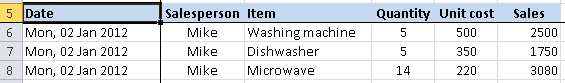
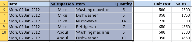
  • Your column headings should occupy just one row of the spreadsheet, as shown in this example:
    ​
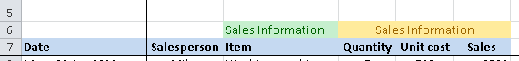
  • You should avoid using column headings in two rows, as shown in the following example, because they can confuse Excel's Autofilter feature and stop it working as it should. While you can still use Autofilter if you have headings in two rows as shown here, it's much easier if you stick to headings in just one row:
    
• Next, make sure there are no empty columns or rows in your data. Excel is good at sensing the start and end of a data table by looking for empty rows and columns, and will ignore data after an empty row or column.
  • A quick tip to check if your data is formatted in one contiguous range (a fancy way of saying "one block of data", which is used a lot in the Excel world) is to click a single cell in the table then press CTRL+* (or CTRL+SHIFT+8 if you don't have a separate number keypad). This automatically selects the whole table. You'll then see if you have any problems with the layout of your table.
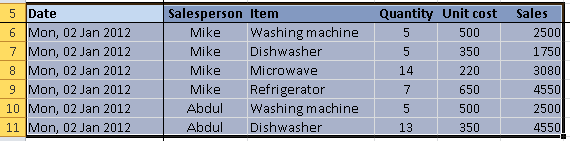
  • This example shows a table that is in a contiguous range:
    
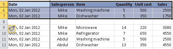
  • This table has an empty row; after pressing CTRL+* to select the table, you can see that the rows after the empty column have been ignored:
    
  • Similarly, this table has an empty column, so the columns to the right of the empty column have been ignored:
    
• • Note that empty cells within the table are OK. What isn't OK is a whole row or a whole column of empty cells.
• Finally, check that you have consistent data types in all cells.
  • For example, if you have a date column, make sure all the values in that column are dates (or blank).
  • If you have a quantity column, make sure all the values are numbers (or blank) and not words.
  • This is not a hard and fast rule, but it will make it much easier to use the features of Autofilter if you follow them wherever possbile.

At this point, if everything is looking OK, you're ready to move on to the next step.

Enable Autofilter

Once your data range that meets the criteria above, you are ready to apply the Autofilter feature:

• Select a cell in the range.
  • Any cell will do, but make sure you don't select more than one cell or Excel will apply the Autofilter to the selected cells rather than the whole table.
  • You may prefer to select all of the cells in the data range if you want - this is a good idea if you have columns with headings in two or more rows (as discussed above).
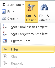
• Next, click the Sort and Autofilter button on the Home tab of the Excel ribbon toolbar, then click Filter.
  
• The first row in the table (the header row) should change, with a small drop-down arrow on each cell in the header row, similar to the example below:
  ​

You are now ready to start using Excel's Autofilter feature.

Using Excel's Autofilter feature to filter your list

You can now filter the table based on the values in the table by clicking the buttons to the right of the column heading. This will show a drop-down list as shown here:

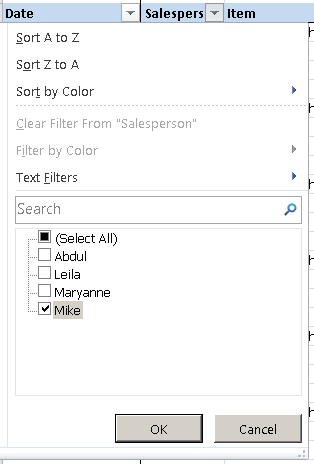
In this example, we've clicked the Autofilter button for the Salesperson. Based on the selection we have made, the list will be filtered to show only rows where Mike is the Salesperson. Other options you have here will allow the following:

• Sorting by Salesperson. In this case the list could be sorted alphabetically in ascending (A to Z) or descending (Z to A) order.
• If you are using Color formatting on the cells in the Salesperson column, you could also choose to sort by Color. This option also hides the very useful (and powerful) Custom Sort option which allows you to sort the list by multiple criteria, such as sorting by Salesperson and then by Item.
• You could also select more than one salesperson from the list by checking the box next to the name of each salesperson you want to filter by.
• Text Filters allow you to use various advanced text filtering options, rather than choosing specific people from the list. One example would be to filter by all salespeople whose name starts with M.
• The Search option is useful when you have a large list of unique records (in this case that would mean lots of different salespeople), so the quickest way to find a specific person is to type their name, rather than scrolling through the whole list. This option was introduced in Excel 2010, and is also available in Excel 2011 for Mac and Excel 2013 for Windows.

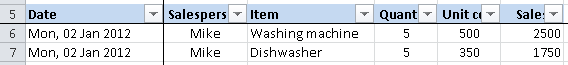
Once you click OK with the selection above, the list will look like this:

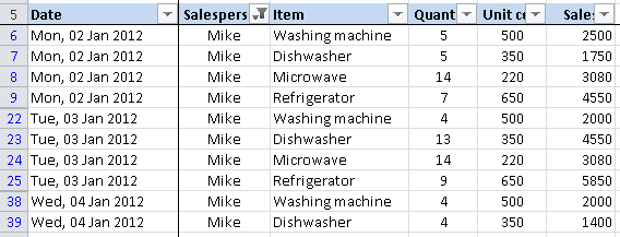
It is important to note two things about this list now that it has been filtered:

• There is a different filter icon at the top of the Salesperson column, indicating that this list has a filter applied on the Salesperson column.
• The row numbers are now shown in blue, indicating that the list has been filtered. Note how the row numbers now skip row numbers for rows that don't match the filter.

This screenshot is just a portion of the full list of sales records for Mike. The Excel status bar at the bottom left of the screen will display the total number of records returned by the filter, as shown here:

Using Autofilter to filter by more than one criteria

The above example used just one criterion - Salesperson - to filter the list. However, you can filter by multiple criteria if you want. For example:

• Show only rows that include sales by Mike, where he sold Washing Marchines (filter by Salesperson=Mike and Item=Washing Machine)
• Show only rows that include sales by Mike where he sold more than 10 units (filter by Salesperson=Mike and Quantity>10)
• Show only rows that include sales of Refrigerators that were made on the 2nd, 3rd or 4th of January.

Once you start working with Autofilter, you will find it an excellent and powerful tool for for filtering and mining data from your spreadsheets. The next lesson will cover more advanced filtering options, and will also show you how to perform calculations that change according to criteria you have used to filter the list.