Find Duplicate Rows in Excel Across Multiple Columns
Excel offers a number of ways to find rows that contain duplicate values. However, most of them focus on finding rows where the value in just one column is duplicated. In this lesson, we look at how to use the COUNTIFS function to find rows with duplicate entries in two or more columns. We then use the COUNTIFS function in combination with Excel's Conditional Formatting feature to highlight duplicate and triplicate rows.
Finding Duplicate Rows - Example data
This lesson uses an example of a product order table. Our data table lists orders of spare parts for several computers. We need to identify how often each spare part is being ordered for each machine. A sample of this data can be seen in the following picture:
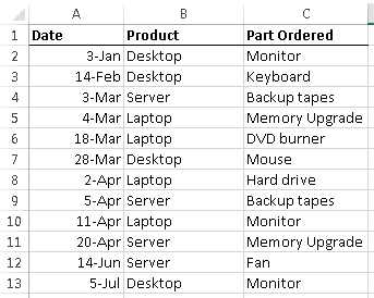
As you can see in this example, there are several examples where the Product and Part Ordered are repeated. For example, a Desktop Monitor has been ordered twice, as have Backup Tapes for the Server.
The COUNTIFS syntax
COUNTIFS is a function that allows you to count only those rows in a spreadsheet where certain criteria are met. It is closely related to the COUNTIF function. COUNTIF allows you to use just one criteria, whereas COUNTIFS allows you to use multiple criteria. You can find out more about COUNTIF in our lesson on how to Use COUNTIF to count the cells in a range that match certain values. Note that the COUNTIFS function was introduced in Excel 2007, so the method we're going to look at in this lesson will only work if you have Excel 2007, Excel 2010 or Excel 2013. The screenshots and examples in this lesson have been produced using Excel 2013, but this method will work in all three versions.
COUNTIFS has the following syntax:
=COUNTIFS(criteria_range1, criteria1, [criteria_range2, criteria2]…)
As shown here, you can define multiple ranges that the COUNTIFS function should look at, and the criteria it should use when deciding whether to count each row as part of its calculation. Our example will require that we use two range/criteria pairs, but Excel allows you to have up to 127 pairs in a single formula.
Use COUNTIFS to find rows that contain duplicate values
The first step in identifying duplicate rows is to write a formula using COUNTIFS to count how often each row is repeated.
We'll start by adding a new column to our table, into which we will enter this formula.
The formula we will use is:
=COUNTIFS(B:B,B2,C:C,C2)
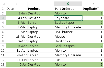
This to be entered into D2 in our table and then copied and pasted down the table. The results of this are shown here:
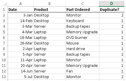
As you can see, there are four rows shown here where the Duplicate value is greater than one. If you look more closely, you'll see that there are actually only two rows which are duplicated (Desktop | Monitor, and Server | Backup Tapes). This indicates that our formula is working, since it has found each row which has a duplicate somewhere in the table.
Let's look a little more closely at the formula we've used:
=COUNTIFS(B:B,B2,C:C,C2)
- Note how we've used B:B to represent the Product column, rather than B2:B13. By doing this, we ensure that our formula will work no matter how many rows we add to the table. We've done the same with C:C to represent the Part Ordered column.
- We've used B2 and C2 to identify the criteria for the COUNTIFS function. Note that they are relative references, so sopying this formula from D2 to the rows below it ensures that the COUNTIFS function always uses the values in the current row as its criteria.
- The COUNTIFS function will only count rows in which both of our criteria are matched.
- Note that if you just wanted to count the rows where only the Product appears multiple times, you would use COUNTIF instead, like this:
- =COUNTIF(B:B,B2)
- This version of the COUNTIFS formula allows you to only show a value in the Duplicates column if the row is a duplicate - in rows that only appear once, nothing will appear in the Duplicates column:
- =IF(COUNTIFS(B:B,B2,C:C,C2)>1,COUNTIFS(B:B,B2,C:C,C2),"") or, even simpler, try this:
- =IF(COUNTIFS(B:B,B2,C:C,C2)>1,"Duplicate,"")
At this point, you may consider your task complete - we've identified the duplicate rows, and we can now use this information to analyse our data further.
Use COUNTIFS to apply Conditional Formatting
However, it may be that we don't want to add another column to identify the duplicates - we only want to identify those rows which are duplicates. We can do this using the COUNTIFS function in combination with Excel's Conditional Formatting feature:
- Click on cell A1. This is important - if you don't, then the Conditional Formatting we are about to set up may be applied to the wrong cells.
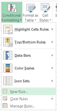
- Create a new Conditional Formatting rule using the Conditional Formatting button on the Home ribbon toolbar:
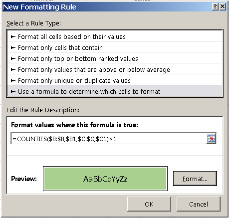
- In the New Rule dialog box, change the values to look like the following:
- There are several points to note when creating the new rule:
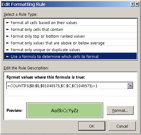
- We are using the option to Use a formula to determine which cells to format. Although Excel offers a Conditional Formatting option to highlight duplicate cells, it won't help us in this scenario.
- The formula that you need to enter in the Rule Description (Format values where this formula is true) is a version of the formula we used in the previous section, but it's critical that you copy it as it's shown here, =COUNTIFS($B:$B,$B1,$C:$C,$C1)>1, otherwise you may get unpredictable results. The $ signs to make the references absolute are needed, as is the change of B2 and C2 in our original formula to $B1 and $C2.
- You can choose whatever formatting you want to appy - I've chosen to fill cells with green shading.
- Once you click OK to this rule, you will need to edit it further to define which cells it should be applied to. You can access the Manage Rules dialog box using the Conditional Formatting menu as shown above (it's the last item in the menu).
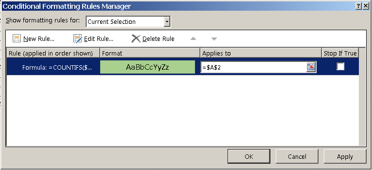
- You should then see the rule you just created in the list - if you don't, change the option shown above from Current Selection to This Workbook and it should appear.
- Change the Applies to value from what is shown above, =$A$2 to =$A:$D. This will tell Excel we want to apply this rule to all cells in columns A through to D.
- You can either type this formula in, or you can click and drag across the row headings to select the rows you want.
- You could also select a specific range of cells, although that will mean you may need to edit this range again in the future.
- You can then click Apply to see a preview of the rule changes in your spreadsheet, or you can click OK to save the changes and return to your spreadsheet, which should now look like this:
- If your spreadsheet looks like this instead, you probably missed the first step in the instructions, which was to click on A1 before creating the rule. In that case, you might see something like this:
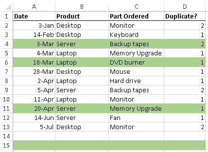
- As you can see, the formatting has been applied to the wrong rows. If this happens, then return to the Conditional Formatting Rules Manager as show above, and edit the rule. You will see something like this:
- Note how the formula we entered has changed (you might see a different formula, but the key is that the criteria values for both ranges have changed). If you see this, it is because you did not have cell A1 selected when creating the rule.To fix this, you can:
- Delete and start the rule, making sure you select A1 before starting.
- Change the formula back to what it should be.
Extending your conditional formatting rules to highlight triplicates and more
In the example above, we created a conditional formatting rule to highlight any rows that are duplicates of other rows, based on a combination of the Product and Part Number fields. You could extend this to cover additional duplicate rule checks - and it's easy to do. To highlight rows that appear three times sor more, do the following:
- Create a new rule using the steps in the previous section. Make it the same as the rule in the example above, with one change to the formula:
- =COUNTIFS($B:$B,$B1,$C:$C,$C1)>=3
- Don't forget to change the formatting you apply to rows that appear three times or more or you won't see any difference.
- Then, change the order of the rules in the Conditional Formatting Rules Manager, like this:
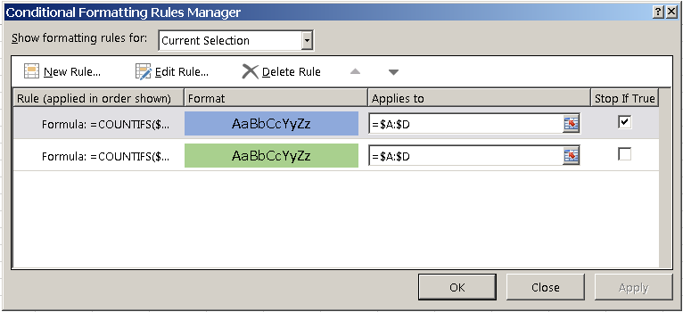
- There are two key points to note here:
- The sequence of the rules can matter. In this case, the triplicate checking rule appears before the duplicate checking rule. If you are trying to create multiple rules to apply to the same range of cells and the formatting is not being applied correctly, it is worth experimenting with the sequence of the rules (there are buttons to move rules up and down next to the Delete Rule button.
- The option to Stop if True can help solve problems in certain cases, if the second and subsequent rules are changing the formatting applied in an earlier rule. This means that the subsequent rules will not be run once the conditions of the first rule have been met.
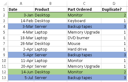
- Here's how the spreadsheet we've been working with looks when you have both rules applied (I have tweaked the data from the original example to include Server | Backup Tapes a third time):
- As a final thought, you could also apply Excel's Autofilter tool to this table. Autofilter allows you to filter based on the colours in a cell, so you could filter out just the green or blue rows. Read our lesson on How to use Autofilter in Excel.
Checking for Duplicate Rows using COUNTIFS - Lesson Summary
In this lesson, we looked at two ways to identify duplicate rows in a spreadsheet, where a row should only be considered a duplicate if the values in two cells match (rather than just one value).
The COUNTIFS function, available in all versions of Excel since 2007, allows us to check for a match of more than one value across all the rows in our table. Unfortunately, it also requires that you create a new column in your table in which to put the COUNTIFS formula; this formula needs to be in every row of your table.
Conditional Formatting lets us take the COUNTIFS function we looked at and use it to apply formatting to rows that are duplicates or even triplicates. We can do this without having to create a new column in our table (note that while we left the Duplicate column in our examples above, we didn't need it there for the Conditional Formatting part of the lesson.
Finally, if you have any questions or feedback on this lesson, please leave a comment below.
Download worked examples
Join our mailing list
Our Comment Policy.
We welcome your comments and questions about this lesson. We don't welcome spam. Our readers get a lot of value out of the comments and answers on our lessons and spam hurts that experience. Our spam filter is pretty good at stopping bots from posting spam, and our admins are quick to delete spam that does get through. We know that bots don't read messages like this, but there are people out there who manually post spam. I repeat - we delete all spam, and if we see repeated posts from a given IP address, we'll block the IP address. So don't waste your time, or ours. One other point to note - if you post a link in your comment, it will automatically be deleted.
Comments on this lesson
Count shows Zeros with Counifs to Find duplicates
Hi There
Very useful articale. I used your way to find and highlight the duplicates. One issue I have is count showing zeros, even when the data is there. I used the below formula in order to avoid comparing against 0 when blank space.
=COUNTIFS(A:A,IF(A2="","",A2),B:B,IF(B2="","",B2),C:C,IF(C2="","",C2),D:D,IF(D2="","",D2),E:E,IF(E2="","",E2),F:F,IF(F2="","",F2),G:G,IF(G2="","",G2),H:H,IF(H2="","",H2),I:I,IF(I2="","",I2),J:J,IF(J2="","",J2),K:K,IF(K2="","",K2),L:L,IF(L2="","",L2),M:M,IF(M2="","",M2),N:N,IF(N2="","",N2),O:O,IF(O2="","",O2),P:P,IF(P2="","",P2),Q:Q,IF(Q2="","",Q2),R:R,IF(R2="","",R2),S:S,IF(S2="","",S2),T:T,IF(T2="","",T2),U:U,IF(U2="","",U2),V:V,IF(V2="","",V2),W:W,IF(W2="","",W2),X:X,IF(X2="","",X2))
Please advice how I can avoide zeros.
Thanks
Baru
highlighting the 2nd duplicate+
Thank you for the lesson.
I am applying this lesson to a list of customers details including phone numbers. The database is provided from multiple sites so when added together their are duplicate records.
What I need to do is highlight duplicates as in the lesson but then find a way to mark the 2nd + duplicate down the spread sheet so the customer only gets called the one time.
Any ideas?
follow on
sorry to add. Using the "remove duplicate" tool in Office 2010 does exactly what I need logic wise apart from it deletes the duplicates completely and I need them highlighted so I can refer back to them in the future.
Duplicate values
This article shows how to highlight duplicate values across a number of columns, however it is looking for duplicate values within each column. I was hoping to highlight cells when the value in the 1st cell in column 1, equals the value in the 1st cell in column 2, and the same all the way down. So if A5=B5 I want it to be highlighted, but not highlight if A5=B6, and not highlight if A5=A6. I hope that makes sense. Is there a way to do this?
Checking duplicates only if entry date is different
Very good lesson, enjoyed reading it and had a good learning. But, what if we want to search for the duplicate entries and want to ignore the duplicate etnries done on the same day
detecting duplicate records and creating a worksheet to exclude
The lesson is clear to follow. How can one create a new worksheet where only a single occurrence of each record exists? I can detect duplicate records (rows) based on criteria applying to a number of columns (in other words the entire record is not duplicated) but I only wish to keep the initial record in each case.
Thank you!!
Thank you so much for providing these instructions. I had no idea where to start. You saved me. Thank you!
Finding Duplicates across multiple columns
I have a less sophisticated way. I also use a helper column called "Duplicate?", but instead of using the countifs function, I use the concatenate function which I copy down to the last row of data. Then I highlight the Duplicate? column and select Conditional Formatting --> Highlight Cell Rules --> Duplicate Values. It is not as sophisticated because it does not display the number of times the entry is repeated, but I find it easier to use especially when there are more than 2 columns of data that I need to compare for duplicates.
Big Thank You!
Just wanna say thank you very much for this! googled for these for past few days but couldn't get the solution until i find this page.
You just save me an hour's work! Awesome and thanks again.
Great Lesson, One Small Correction
You can have multiple criteria, but when you have just one, it's called a criterion. ;P
HIGHLIGHT ONLY A DUPLICATE NOT ALL
Can i ask how to highlight only a duplicate instead of all.
For example:
1 1 1 1 1 1 1 1
0 1 0 0 0 0 0 0
0 0 0 0 0 0 1 0
1 1 1 1 1 1 1 1
2 2 2 2 2 2 2 2
2 2 2 2 2 2 2 2
3 3 3 3 3 3 3 3
3 3 3 3 3 3 3 3
There is duplicates between row 1&4, 5&6, 7&8. But i need to highlight only row 1, 5 and 6. How? Can you teach me?
Thank you!
correction:
correction:
highlight only row 1, 5 and 7
Find Duplicate Rows in Excel Across Multiple Columns and divide
Find Duplicate Rows in Excel Across Multiple Columns and divide
Conditional Formatting looking for duplicates in sports fixtures
I am trying to edit this formula so it will work for an excel document of sporting fixtures. This league has more teams than rounds so I don't want any team to play each other twice or more in a season.
I have followed the above steps. It works if I make an exact copy of a previous fixture (e.g. if Round 1 = A vs B and Round 5 = A vs B both rows highlight).
How can I edit it so it would also pick up if Round 1 = A vs B and Round 5 = B vs A?
Basically I need it to highlight the cell if there is a duplicate fixture, regardless if the home and away team have swapped for the second fixture
Counting more than one column matching multiple criteria
Hello,
I'm looking to find the sum of how many people show up on multiple cases. IE: =1, =2, =3, >3 (listed separately)
Employees w/1 case=
Employees w/2 cases=
A2:A211 is case #, B2:B211 is Employee #. An employee may be listed multiple times under the same case # and in multiple cases.
CASE # EMP #
111 900
111 900
111 901
112 900
112 902
113 903
114 900
The answer for Emp #900 = >2.
Can Excel copy the emp # to a separate list?
IE: Employees w/2 cases = 2
900
905
Your help is much appreciated.
re: how to highlight column G,H,I& J all have 0 value(same row)
I did a lot of google search, your lesson is the best close solution for my issue. i have excel sheet with over 1000 rows and 12 columns. what I need to find out is that 4 columns all have 0 value at the same time. those 4 columns are currency $ value. I need to highlight the row if all 4 columns have "0" value at the same time.
can you please teach me? it's too hard to manually highlight row by row. thank you so much. Adriana
For removing duplicated numeric from excel multiple arrays
If for numeric data, I use different method to remove duplicated values in multiple arrays, say A2:C10:
1. Sort columns data (A2:C10) in ascending order with "Sort By" condition for each columns
2. Input default value = 1 at new column (E2) for row A2
3. Subsequent rows (A3:A10) at new column (E3:E10), add-in with formula =IF(SUMPRODUCT(ABS(A3:B3-A2:A2))>0,1,0)
4. If current array data match with the one on top, the formula will give a 0 to denote duplicated data
5. Copy all values only from this new column (E2:E10) to another new column (D2:D10)
6. Sort this new column (D2:D10) first in descending order follow by all array data (A2:C10)
7. In this way, all non-duplicated data will be put on top of the list
8. Use formula =CountIf(D2:D10,">0") to get the number of total non-duplicated values
Dose for Excel Add-In
You can use Dose for Excel Add-In that includes an awesome features to highlight or delete duplicated rows besides more than +100 new functions and features to add to your Excel to save time and effort.
Duplicate rows from one sheet to another
Hello, excellent information!
However, I have two sheets in one workbook that I need to compare. all of the column names are identical to each other and in the same order. I need to know if the data in Sheet1 A2 to BU2 has a duplicate row in anywhere in Sheet2 A to BU. There are literally over 100,000 rows in Sheet1 that I need compared to Sheet2.
Any thoughts?
Thank you.
Dan
Finding Duplicate with conditions
a guest must pay only one day rent for 1 bed only.
There are few guest repeated twice in a day in different room. help me identify the duplicate to avoid extra payments to hotel
Cannot Get Formula to Work Unless Row #s Same
I followed the instructions here to build a formula to identify duplicates in which the three first columns are an exact match for a row across two sheets. Unfortunately, it only seems to work if the duplicate rows are the same row number on both sheets. Is there a way to identify duplicates that match three columns of data (eg: client name, order number, client ID are all the same on two sheets)? What am I missing?
Here's what the formula looks like:
=IFERROR(VLOOKUP(A2&B2&C2,IF({0,1},WG!N$2:N$4999,WG!A$2:A$4999&WG!B$2:B$4999&WG!C$2:C$4999),2,0),"Not a Duplicate")
WG is the name of the sheet where the reference column with 1 in it is located.
Any help or advise is most welcome!!!
Thanks,
Greg
Finding rows that contain duplicate values
Hello, I think the COUNTIF or COUNTIFS functions using will work well for what I am trying to do. However, there are blank cells in the range that are being counted as duplicates. Can you explain how to alter the formula to exclude blank cells from the COUNTIF function?
Thank you for sharing this great lesson. Take me more than 5 minute to learn but well worthy!