Calculate a running total of a column of cells in Excel
If you have a column of numbers and you want to calculate a running total of the numbers in each row, you have two options open two you:
- You can create a simple addition formula
- You can write a formula using the SUM() function which utilizes absolute and relative references.
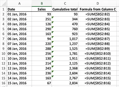
Imagine your spreadsheet has values in cells A2 through to B16. You want to put a running total of sales (column B) in column C:
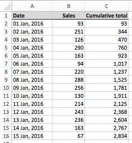
As you can see, column C shows the cumulative running total of the sales in column B.
Option 1 - create a simple addition formula in the second row, and copy it down the column
To use this method, you need two simple formulas
First, enter this formula into C2 (using the example above)
=B2
Then, in C3, enter this formula:
=C2+B3
Finally, copy and paste the formula from C3 into C4, C5, C6 and so on down the column.
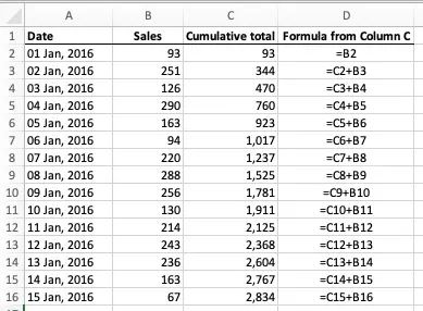
You should end up with a spreadsheet that looks like the example below. Column D shows the formulas that have been entered into column C.
- Cell C2 is equal to the value in B2
- C3 takes the value in C2 and adds the value in B3. This is the running total so far.
- C4 takes the value in C3 and adds to it the value in B4 to get the running total for row 4.
- This continues down the table.
This method works well, but has one key limitation. The spreadsheet is currently sorted by Date. If you sort the table of data by a column other than Date, such as Sales, the formula will break. This is because all the values from cell C3 downwards rely on the value in C2. If the value in C3 is moved elsewhere in the table, the running totals will no longer calculate correctly, as you'll see in the example below. The table has been sorted by Sales, from the smallest sales to the largest, and the formula that was in B2 is no longer first in the list. The result in this example will look like this:
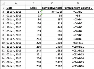
As you can see, there is a #VALUE error in C2. Also, the formula that was in C1 is now in column C2, so the value in B2 is no longer being included in the overall total.
Notice how the formula in C2 now tries to add the value in C1 to the value in B2. The #VALUE error in C2 indicates that the formula cannot calculate a result because of a problem with the values in the cells it is referencing. In this case, the problem is that C1 contains words, not numbers.
Notice how this table changes if we sort it so that Sales go from largest to smallest:
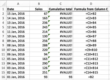
In this example, the long list of #VALUE errors means you could be forgiven for thinking that your whole spreadsheet has been broken. However, all that has happened is that the formula that was in the first row of data is now last. All of the other formulas are returning a #VALUE error because of the formula in C2, which attempts to add words to a number. The formula in C3 then tries to add #VALUE to a number, which also return a #VALUE error - so the problem cascades down to the end, where the formula in C16 finally returns a number - the value in B16.
Option 2 - use the SUM function with absolute and relative references
Let's look at another method of calculating a running total that doesn't have the same problem when it is sorted. This method works because of the way it uses the SUM function plus a combination of absolute and relative references.
Here's our original example, with column D now showing that a different formula is being used in column C:
To reproduce this you would do the following:
- In cell C2, enter the following formula:
- =SUM($B$2:B2)
- This will put the value of B2 into C2. The SUM function here is adding up all the cells between $B$2 and B2 - which is just one cell, B2.
- Remember that $B$2 is an absolute reference. This means that anywhere you copy this formula, it will always refer back to B2.
- Then, copy this formula and paste it into cell C3. The formula should now look like this:
- =SUM($B$2:B3)
- This will put the sum of all the cells between B2 and B3 into C3.
- Note that, as promised, $B$2 hasn't changed even though you have copied the cell from one place to another.
- On the other hand, B2 was a relative reference in the previous cell, so it changed from B2 to B3 when you copied and pasted the formula from C2 to C3.
- Once you've verified that this works as described, you can then copy the formula into each cell from C2 to C16. The final cell, C16, will contain the total of all the numbers in the cells from B2 to B16 (i.e. $B$2:B16).
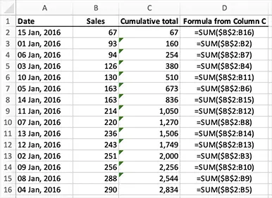
Now, let's check what happens if we sort this table. The following two examples show the table sorted first from the lowest Sales value to the highest, and then sorted from the highest Sales value to the lowest, just as in Option 1. This time, however, the running total still works, with no #VALUE errors:
Sales lowest to highest - formulas continue to refer back to B2 as the starting point
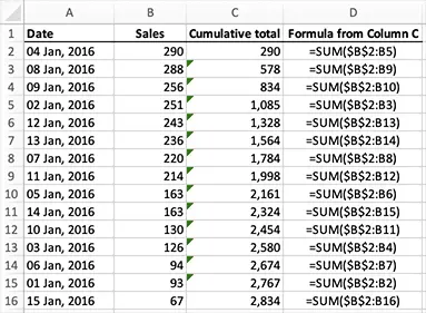
Sales highest to lowest
Note that there are some scenarios where a formula like this is more than you need. Check out this comment to see another way to do it that allows to calculate a running balance based on two columns of numbers.
Finally, a common requirement is to calculate a running total based on data between two dates. Click the link to see now to do this.
Do you have any questions about on this lesson, or a specific problem you need to solve? If so, please leave a comment below.
Join our mailing list
Our Comment Policy.
We welcome your comments and questions about this lesson. We don't welcome spam. Our readers get a lot of value out of the comments and answers on our lessons and spam hurts that experience. Our spam filter is pretty good at stopping bots from posting spam, and our admins are quick to delete spam that does get through. We know that bots don't read messages like this, but there are people out there who manually post spam. I repeat - we delete all spam, and if we see repeated posts from a given IP address, we'll block the IP address. So don't waste your time, or ours. One other point to note - if you post a link in your comment, it will automatically be deleted.
Comments on this lesson
Thank you
Fantastic tutorial, I can use excel but had never done a running total, it took me about 30 seconds of reading to understand what to do....far better than microsoft help page!
Nice little trick. We'll
Nice little trick. We'll explained. Saved lot of tome for me. Thanks for posting this useful tip. God bless.
running total amount in excel
The Total Amount is incrementing(single cell:H2) when value is entered in the same cell(G2)..e.g today if you enter in G2 the value of 30 the total amount in H2 is 30;when you enter tomorrow in G2(same cell) the value of 50, the total amount in H2 should be 80;and when you enter again 80 in the same cell(G2)the next day, the total amount should now be 160...hope you could shed a light on this...Thank you very much...
i'm sorry..i posted a comment
i'm sorry..i posted a comment that should be query...
Running Total
Thank you for posting this. It worked perfectly.
find Cumulative total of column with large vol different items
Month numbers Tno Name PF own PF co cum own cum co
Sep-13 1 335 Mr A 13598.00 13057.00
Oct-13 2 335 Mr A 14099.00 13558.00
Nov-13 3 335 Mr A 14099.00 13558.00
Dec-13 4 335 Mr A 14099.00 13558.00
Jan-14 5 335 Mr A 14099.00 13558.00
Feb-14 6 335 Mr A 14099.00 13558.00
Mar-14 7 335 Mr A 14099.00 13558.00
Sep-13 1 338 Mr B 13598.00 13057.00
Oct-13 2 338 Mr B 14099.00 13558.00
Nov-13 3 338 Mr B 14099.00 13558.00
Dec-13 4 338 Mr B 14099.00 13558.00
Jan-14 5 338 Mr B 14099.00 13558.00
Feb-14 6 338 Mr B 14099.00 13558.00
Mar-14 7 338 Mr B 14099.00 13558.00
excel formulas, combinations, etc
thanks. Long, I have been searching for a formula. I could explain the problem too. But, today, I got it. thank you. In future, I may request your help.
Complete Column
That works great. It solved my no reference error for the first line, which i need to apply for the whole column (STRG + D).
Thanks!
I'm so happy to have a resource like this available to me! I finally figured out how to use the pesky $ sign in my formulas. Thank you internet stranger!
Hi I seem to have stumbled
Hi I seem to have stumbled across a problem that I simply can't find the answer to. I want to have a running total against the days of the month (so a full year would be 365 lines). Income and outgoings, and the total. I can make the sum of two cells as above, but I can't seem to figure out how to make that cell, for example, D2 carry onto D3/4/5 and only being adjusted by the income and outgoings (B and C). I'd be hugely appreciative if you have a solution, I'm fairly sure it's an easy one but I simply don't have any experience with Excel.
I think the solution you need is simple
Hi Dan
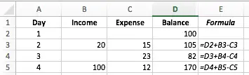
While you could use the approach shown in this lesson, it sounds like you need a simple formula that looks something like this:
=D2+B3-C3
In this formula, I'm assuming the following:
- This formula will be entered into D3
- D2 (the cell above) contains your opening balance. This will need to be manually entered.
- B3 contains Income.
- C3 contains Expenses.
Essentially, this formula says "take the balance from the previous row, add the income for today and subtract the expenses for today". It will be more efficient and therefore faster than a formula that tries to calculate a running balance based on income and expenses, especially as your spreadsheet gets bigger.
You'd then copy and paste this formula down column D to the end of your table.
Here's an example. Column E shows the formulas from column D:
Some additional thoughts ....
- There's no reason not to have multiple rows for a given day.
- I'd make sure that there is a column with the number of the day or the actual date.
- Then, you can add multiple rows for each day, and sort them by the day/date column.
This approach is useful for reconciling a bank statement, for example, which can have multiple in/out transactions (or no transactions at all) on a given day
You're right, that formula
You're right, that formula sounds exactly what it is. Feel a bit silly now for not realising. Thanks millionleaves :)
Hi
Hi
Do you have the formula that will work, as that just says there is a circular error. I think it's more like C3:B3 but then I'm stuck. I still can't get it to take the previous running total into consideration.
The formula shown in the image is correct
Hi Dan
The formula in the image that I posted is the correct formula.
If you're getting a circular error, you may be using a different formula, e.g.
=D3+B3-C3
If you put this formula in D3 it will generate a circular error since it is trying to add itself to itself.
The correct formula in D3 is this:
=D2+B3-C3
Note that the formula in D3 refers to the cell above it - D2 - to get the previous balance.
Thanks again, I think I've
Thanks again, I think I've found it now, it must be my version of Excel or something, it's this =SUM(D1,B3:C3)
Running balance
I've started maintaining a bank balance sheet on Excel. There are the debit, credit and balance columns. I have plugged in a formula in the balance column as such: previous balance + debit - credit. It works fine, but I would like to have that formula running down that entire balance column. When I do a Fill Down, it fills the formula in but the value is also there. I would like for the end result to not show up until the row is filled with values. So only when I have a transaction should the balance for that row show up. Thoughts? Thanks.
I like how this is going, but...
What I would like to know is if there is a way to get your final result (say D5 in this instance) to just be in one cell instead of the whole column? So it could just sit around E3 or something? It would make the worksheet look more tidy for my needs.
won't calculate zeros
I do a daily total of sales. If there were no sales for the day, and "0.00" is entered into the cell, it puts "0.00 into the subtotal column. I need the total for the last day to populate that days running total. How can I force the system to ignore the zero. I always thought that you just entered a condition like =(IF(C18,1,0))*SUM(C$2:C18) What am I doing wrong. If you could help, I would really appreciate it.
Thank you!
Sorted rows running total
How would you get a correct running total for just the rows that are sorted. Ex I need costs of just travel, but main formula is total costs. Lodging, flights, food etc.
Sorted rows running total
How would you get a correct running total for just the rows that are sorted. Ex I need costs of just travel, but main formula is total costs. Lodging, flights, food etc.
Cumulative formula
I created this one just now =SUM(INDIRECT("D4:"&"D"&ROW())) - numbers start at D4.
Running total
Hi
Looking to create a table of data, that has an accumulative figure for the month. But I want to exclude any data for days that doesn’t meet the required number, in this instance data less than 0. I don’t want a negative number to effect the running total.
Any help for a novice spreadsheet user.
Running total
Hi
Looking to create a table of data, that has an accumulative figure for the month. But I want to exclude any data for days that it doesn’t meet a required number, in this instance data less than 0. I don’t want a negative number to effect the running total.
Any help for a novice spreadsheet user.
YTD Total Cell
I had to create a paycheck on excel and enter my numbers manually (don't ask, long story with accountant) and I am wanting a cell to automatically update with the YTD amount if possible.
Currernt YTD
NET PAY $944.28 $944.28 (can i use a formula that would take $944.28 and add the current $ amount automatically? and then next week it would take the Current $ amount and add it again to stay current) or do i have to enter it manually.)
Weeks ago i emailed
Weeks ago i emailed Robinsonbuckler (( @yahoo )). com to restore my relationship and he did after 24 hours…
Running Total in Table
While this formula works, I run into issues when used in an expandable table. Excel does unexpected things, such as skipping a cell in its calculations. Any advice?
cure herpes
I was having Herpes Simplex Virus then i came across a review of people saying that they got treated from Herpes Simplex Virus by Dr Voke., So i gave a try by contacting him through his email and explain my problem to him. He told me all the things I need to do and also give me instructions to take, which I followed properly. Before I knew what is happening after two weeks the HERPES SIMPLEX VIRUS that was in my body got vanished . so if you are also heart broken by any deadly diseases like HERPES HIV, shingles,low sperm count or bringing back your ex lover, this great man is extremely the best in which I have seen and applauds and if you also need a help, you can also email him via email doctorvoke @gmail .com
Anna
if you enter in G2 the value of 30 the total amount in H2 is 30;when you enter tomorrow in G2(same cell) the value of 50, the total amount in H2 should be 80;and when you enter again 80 in the same cell(G2)the next day, the total amount should now be 160...hope you could shed a light on this...Thank you very much...
Herpes cure
Was cured from herpes virus. thanks to R.buckler 11 [at] G mail com………………..
HERPES CURE
I was browsing the Internet searching for help when I came across a testimony shared by someone on how she was cured from Herpes Disease. I quickly contacted him to get the cure. I bought the herbal medicine from the herbal doctor [Robinson Buckler]. I took the herbal medicine for 2 weeks as instructed and i went for a medical checkup and to my greatest surprise i was cured from Herpes virus. My heart is so filled with joy. If you are suffering from Herpes or any other disease you can contact this herbal doctor today on this Email address_________________robinsonbuckler @[[yahoo .com]].....Thank you Doctor
Robin Burroughs
Denton Avenue
Cookeville, TN 38501
USA
Very nicely worded. I like being able to understand what I'm doing, instead of just copy/pasting