If you're getting started with Excel, creating formulas is one of the first things you should learn. In this lesson you'll learn how to create simple formulas and calculations in Excel.

At its heart, Excel is a giant calculator. In fact, a simple way to think about Excel is to consider each cell in a worksheet like an individual calculator. An Excel spreadsheet has millions of cells, which means you have millions of individual calculators to work with. Not only that, but you can create formulas that link different cells together (e.g. add the value in this cell to the value in that cell). You can create formulas that link cells in different worksheets together. And you can even create formulas that link cells in different workbooks together.

How to enter a formula in Excel

In Excel, each cell can contain a calculation. In Excel jargon we call this a formula. Each cell can contain one formula. When you enter a formula in a cell, Excel calculates the result of that formula and displays the result of that calculation to you. In fact, when you enter a formula into any cell, Excel will recalculate the result of all the cells in the worksheet. This normally happens in the blink of an eye so you won't normally notice it, although you may find that large and complex spreadsheets can take longer to recalculate.

When entering a formula, you have to make sure Excel knows that's what you want to do. You start by typing the = (equals) sign, then the rest of your formula. If you don't type the equals sign first, then Excel will assume you are typing either a number or a text. You can also start a formula with either a plus (+) or minus (-) symbol. Excel will assume you're typing a formula and insert the equals sign for you.

Here are some examples of some simple Excel formulas and their results:

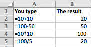
In this example, there are four basic formulas:

• Addition (+)
• Subtraction (-)
• Multiplication (*)
• Division (/)

In each case, you would type the equals sign (=), then the formula, then press Enter to tell Excel you've finished.

• Sometimes Excel will show you a warning rather than just entering your formula. This will happen if the formula you've typed is invalid, i.e. is not in a format that Excel recognises. It will usually also give you some indication of what you did wrong.
• Other times, Excel may enter the formula you have typed correctly but then show you an error such as #VALUE. This means that you have entered a formula that was value, but Excel could not calculate a valid result from your formula.

Creating formulas that refer to other cells in the same worksheet

Excel's power comes from allowing you to create formulas that refer to the values in other cells.

In the example above, you'll notice the headings across the top (A, B) and down the left (1,2,3,4,5). By comining these values, we have a unique reference each cell in a worksheet (A1, A2, A3, B1, B2, B3, and so on).

When you create a formula, you can refer to other cells using these cell references to incorporate the values in other cells into a formula. The value in another cell might be a simple number, or another cell containing a formula. When you create a formula that refers to another cell that also contains a formula, your formula will use the result of the formula in that other cell. Then, if the result of the formula in that other cell changes, so too does the result in your formula.

Here are some examples of some Excel formulas that refer to other cells:

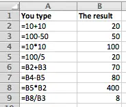
In this example, rows 6-8 build on the earlier examples to link cells together:

• B6 adds the values in B2 and B3 together. If you change either of the values in B2 or B3 the result in B6 will change too.
• B7 and B8 subtract and multiply the values in other cells.
• B9 goes a step further and divides B8 by B3. Note that B8 in turn multiplied B5 and B2 together. So changing the values in either B5 or B2 will have a domino effect, where the value in B8 will change, and so the value in B9 will change too. Note that Excel handles all of this the moment you finish entering a change in either B5 or B2.

Creating formulas that refer to cells in other worksheets

When you first open Excel, you start with a single worksheet. However, Excel allows you to have more than one worksheet inside a single spreadsheet file (known as a workbook). In fact, in earlier versions of Excel a new workbook automatically started out with 3 worksheets inside it.

Earlier we saw how to link two cells together within a worksheet by referring to other cells using their cell reference value. Referring to a cell inside another worksheet works in much the same way, but we need to provide more information about the location of that cell so Excel knows which cell we're talking about.

Here are some examples of formulas that refer to cells in another worksheet inside the same workbook:

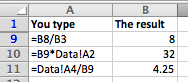
In this example, the formulas in B10 and B11 refer to cells in another worksheet called Data.

• B10 multiples the value in B9 by the value in cell A2 in the worksheet called Data
• B11 takes the value A4 in the worksheet called Data and divides it by the value in B9.

In other words, we've told Excel to go to the worksheet called Data and use values in that worksheet in our formulas.

There are a couple of ways to create formulas like this:

• Type the formula in by hand. In the above example, you would create the reference to the other worksheet by typing the worksheet name followed by an exclamation mark (!); the exclamation mark tells Excel that you're referring to another worksheet.
• Start typing the formula by typing the equals sign (=), then click on the name of the other worksheet. Excel will switch to the other worksheet, and you can click on the cell you want to reference in your formula. You can then press Enter to finish entering the formula, or you can click back on the original worksheet name and finish typing your formula before pressing Enter.

Note that if you rename the worksheet called Data, the formulas that refer to Data will automatically update to reflect the new name. Here's what the above examples look like if we change the name of the worksheet called Data to Daily Data.

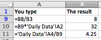
Note how Excel has put apostrophes around the name of the worksheet called Daily Data. This is because of the space in the worksheet name. Excel does this to make sure that the reference still works; if you manually type the formula without the apostrophes then Excel will not be able to validate the formula, and will not let you enter it.

Creating formulas that link to other workbooks

As you might imagine what we've already covered, it is also possible to create a formulat that refers to cells in another workbook (i.e. another file). Once again, it's simply a matter of correctly referring to the cell in the other workbook.

The following example shows what this looks like:

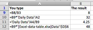
In this example, B12 contains a formula that refers to cell D6 in a worksheet called Data in a file called Excel-data-table-xlsx.

• The square brackets are used to indicate the filename, i.e. [filename]. Be aware that if the file referred to is not currently open, the square brackets may also include the full file path to that file, so that Excel can still read the value from the cell being referred to even though the file is not open.
• The apostrophes are used to enclose the full file name and worksheet name.
• Then, Excel uses absolute references to identify the cell being referred to. This means that if you move (not copy) the contents of cell D6 in the Data worksheet, your formula will still work. The $ signs are used to denote an absolute reference (as opposed to a relative reference). Absolute and relative references are out of scope for this lesson, but you can read about them in this lesson.

Summary

Learning to use Excel formulas is one of the most important things you'll learn to do with Excel. Hopefully this lesson has set you on the right path, and you'll be creating spreadsheets with formulas of your own in no time at all. If you have any feedback or questions on this lesson, please comment below!