The SUMPRODUCT function allows you to multiply two columns or rows of numbers together (e.g. Quantity Sold and Price Per Unit) and add the results of each individual calculation together. Without the SUMPRODUCT function, you would have to to create a third column or row in which you write a formula to multiply the Quantity by Price for each entry in your data, and then write another formula to find the sum of all of those numbers. You can also use SUMPRODUCT with one or multiple criteria, whereby SUMPRODUCT will only operate on rows that meet the criteria you define.

This lesson shows you how to use SUMPRODUCT to do all this, with just one formula.

Scenarios where SUMPRODUCT is useful include:

• Finding the total sales for all products, where you have Quantity Sold in one column and Price per Unit in another.
• Finding the total sales for all products, but only include those sales for a specific City (i.e. specify criteria for SUMPRODUCT)
• Finding the total sales for all products, but only include those sales for a specific City and Day (i.e. specify multiple criteria for SUMPRODUCT)

We'll cover examples of all three scenarios in this lesson.

SUMPRODUCT Syntax

The syntax of the SUMPRODUCT function is as follows:

=SUMPRODUCT(array1, [array2], [array3],...)

where array1 is the data in the first column, array2 is the data in the second column and so on.

Some points to note:

• You only need array1 for the function to work BUT if you only have array1 then SUMPRODUCT works the same way as SUM
• Array2 and Array3 are both optional. In fact, you can have 255 arrays in one SUMPRODUCT formula
• However many arrays you have, they must all be the same shape. You can't have array1 containing 43 cells in a column, and array2 having only 42 cells - Excell will return a #VALUE error.
• If any cells have text in them, the SUMPRODUCT functions treats them as containing zeros.
• As we will see later, you can incorporate a logical test into each array value to emulate the way that SUMIF or SUMIFS works.

Using SUMPRODUCT in a simple example.

Let's look at how to use SUMPRODUCT in a simple example. This is how most people use SUMPRODUCT.

• In this example, we'll use the following example where we want to find the total value of sales for Monday:
  
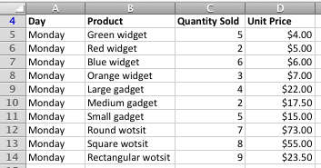
• As you can see, we have a range of products on sale at different unit prices. Without SUMPRODUCT, we would have to add a new column to find the sales for each product, and then add up the results of that column to find total sales.
• In this case, we'll enter the SUMPRODUCT formula in a cell below the table:
  
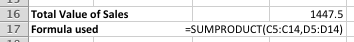
• As shown here, the formula is =SUMPRODUCT(C5:C14,D5:D14). As you can see, the formula includes two arrays:
• • An array (range of cells) that contains the quantity sold.
  • An array that contains the unit price
• Our SUMPRODUCT formula works by multiplying the quantity by the unit price for each row, and then returning the total for all rows in our array.

Bear in mind that this is a simple example that only uses two arrays - quantity and price - to find the result we want. It's worth remembering at this point that we can use more than two arrays if we wanted to.

Using SUMPRODUCT with criteria

Let's now expand our simple example. Let's say we want to specify some criteria for the SUMPRODUCT function so it only adds up the sum of some of the rows. In other words, we'll use SUMPRODUCT to find a subtotal of our data based on our criteria.

• Let's say we have another sales report for Green Widgets which breaks down our sales by city as well as by day, as shown here:
  
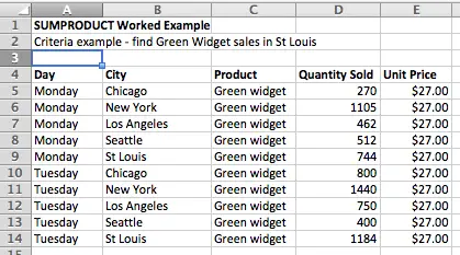
• We would like to find the sales of Green Widgets for St Louis.
  • In other words, we want to use SUMPRODUCT to find the value of sales of Green Widgets, with the additional criterion that we want to include only those sales of Green Widgets made in St Louis.
• We can expand the SUMPRODUCT function by changing one of the arrays to include a test to see if the City is St Louis, as show here:
  
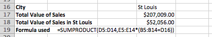
• Let's look more closely at this formula, =SUMPRODUCT(D5:D14,E5:E14*(B5:B14=D16)). As in the previous example, we have two arrays:
  • The first array, D5:D14, is the same, and contains the data for quantity sold.
  • The second array, E5:E14, is different. It contains the unit price, but it then multiplies the value in the Unit Price column by a logical formula, B5:B15=D16.
  • This logical formula works by comparing the City value (column B) in each row with the value in D16 (St Louis). If the value in the City colum is St Louis, the logical formula returns 1, otherwise it returns 0.
  • Multiplying the price by the result of this logical formula by the quantity sold for each row means that any row where the City is not St Louis will have a value of zero when SUMPRODUCT adds up the products of all the rows.
  • We have achieved our objective - we have used SUMPRODUCT with a criteria of "City = St Louis". The result can be see in the field "Total Value of Sales from St Louis.
  • You can download the spreadsheet we used for this example here.
  • You can read more about logical formulas in our lesson Using logical operators and functions in Excel
• It's important to note that it doesn't matter where in our formula we use the logical formula to check if the City value is St Louis. We used Price, but using Quantity would have yielded the same result. Here's what that formula looks like::
  • =SUMPRODUCT(D5:D14*(B5:B14=D16),E5:E14)

Using SUMPRODUCT with criteria in this way allows us to find the answer we want using a single formula. The alternative approach would be to add another column in which we calculate the sales for each row by multiplying Quantity Sold by Price. We could then use the SUMIF function to add up the numbers in that column that match our criteria that the city must equal St Louis. As you can imagine, this requires more work than using the SUMPRODUCT function with a criterion as we have seen it here. You can learn more about SUMIF in this lesson: Using SUMIF to add up cells in Excel that meet certain criteria

In our next example, we'll look at how we could use more than one criteria with SUMPRODUCT.

Using SUMPRODUCT with multiple criteria

For our next example, let's extend our example to have SUMPRODUCT emulate the SUMIFS function. SUMIFS allows you to add up a row or column of numbers, but only include those values where two or more criteria are satisfied. You can read more about the SUMIFS function in this lesson: Use SUMIFS to sum cells that match multiple criteria in Excel.

• In this case, we would like to find the total value of sales for Green Widgets sold in St Louis on Tuesday:
  
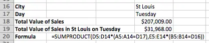
• Our formula now looks lie this: =SUMPRODUCT(D5:D14*(A5:A14=D17),E5:E14*(B5:B14=D16)) so that we are only :
  • The first array, D5:D14*(A5:A14=D17), will return the quantity sold if the Day is Tuesday (i.e. the value in D17), or zero if the day is not Tuesday.
  • The second array, E5:E14*(B5:B14=D16), will return the unit price if the City is St Louis (i.e. the value in D16), or zero if the city is not St Louis.
  • In other words, only rows that include Day = Tuesday AND City = St Louis will be included in our total.
• Finally, if you wanted to find the total value of sales for Green Widgets sold in St Louis OR Chicago on any day, you could use this formula:
  • =SUMPRODUCT(--((B5:B14="Chicago")+(B5:B14="St Louis")),D5:D14,E5:E14)
  • This formula checks to see if the City column contains Chicago or St Louis and returns 1 if either are found, and 0 if neither are found. This result is multiplied by the Quantity and Price columns to give the result.

Summary of this SUMPRODUCT lesson

In this lesson we looked at how SUMPRODUCT can save a lot of time when trying to summarise data in a spreadsheet. Specifically, we were able to use it to write one formulat that will find the total sales in a data table that includes Quantity Sold and Unit Price, without having to create a new column to find the total sales value for each row.

We also looked at how to use SUMPRODUCT with one or more criteria to find the total sales in our example, but only for those rows that met the criteria we specified. In our examples, we first found the total for all rows that matched a certain City, and for those rows that matched a certain City AND Day. We also considered the use of SUMIF as an alternative to using SUMPRODUCT, and realised that it would involve writing multiple formulas to achieve the same result.

If you have any questions about how to use SUMPRODUCT in other ways, or you have feedback on this lesson, feel free to add a comment below.