Use Conditional Formatting to shade alternate rows in Excel
If you are working with large tables of data in Excel, you can make your spreadsheet easier to read by formatting alternate rows to be shaded a different colour. There are a number of ways you can achieve this. This lesson shows you a quick and easy way to do it on Excel 2011 for Mac.
Configure alternate row shading in Excel 2011 for Mac
This method uses the conditional formatting option in Excel that allows you to set the format of a cell or range of cells based on the outcome of a formula. The way it works is to check to see if the current row number is an even number, and then format the even numbered rows with a formatting colour/shading of your choice. It is a bit convoluted, but works well once you follow these steps.
- Select the range of cells you want to format with alternat row shading.
- Click the Conditional Formatting button on the Home menu

- Then, click the option you want from the drop down list. In our case, we are skipping the presets (the first five options) and setting up a New Rule.
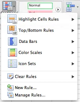
- Note that you can also choose Conditional Formatting from the Format menu.
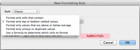
- The New Formatting Rule dialog box will then be displayed as follows. The dialog box defaults to 2-color Scale. In our case, we need the Classic option from the list shown in the screenshot below:
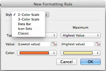
- Once you have chosen the Classic formatting rule style, the New Formatting Rule dialog will change to show you the related options:
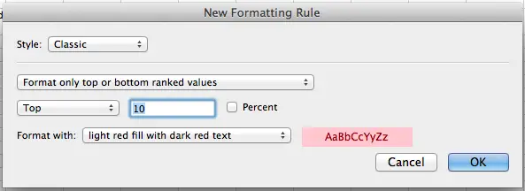
- Next, change the formatting option from the default of Format only cells that contain to Use a formula to determine which cells to format, which is the last option shown in the dialog box below:
- Finally, configure the options to look like the following screenshot.
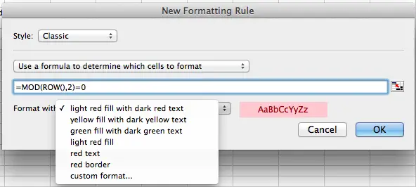
- You should have entered the formula as shown, and then selected a formatting option from the Format With dropdown box.
- The formula shown, =MOD(ROW(),2)=0 checks to see if a row is an even numbered row
- The Format With option lets you choose from several pre-set formatting rules (we'll choose green fill with dark green text for our example) or to choose a custom format.
- Once you've finished configuring the conditional rule as shown above, click OK to save the new rule. The Manage Rules dialog will appear:
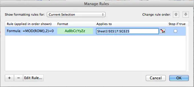
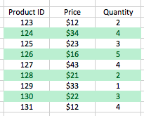
- As you can see, this rule will be applied to the range selected. Click OK once more to see how the selected cells look once the rule is applied:
- If you want to modify the rulem, you can get back to the Manage Rules dialog box by choosing Conditional Formatting from the Formatting menu.
Join our mailing list
Our Comment Policy.
We welcome your comments and questions about this lesson. We don't welcome spam. Our readers get a lot of value out of the comments and answers on our lessons and spam hurts that experience. Our spam filter is pretty good at stopping bots from posting spam, and our admins are quick to delete spam that does get through. We know that bots don't read messages like this, but there are people out there who manually post spam. I repeat - we delete all spam, and if we see repeated posts from a given IP address, we'll block the IP address. So don't waste your time, or ours. One other point to note - if you post a link in your comment, it will automatically be deleted.
Comments on this lesson
I agree. These instructions
I agree. These instructions were clear and complete.
Don't pay attention to the naysayers
You've provided excellent instructions. Thanks for taking the time and effort to share them. Greatly appreciated.
Thank you, just want I needed
Thank you, just want I needed for the Mac, kept getting PC instructions...
You would think Microsoft would just make this a one click option...
Error
I seem to get an error message onc ei enter this function any insights? im copy pasting the rule into the bar but still getting an error
thank you!
thank you
I'm really grateful for this lesson. Thanks so much for taking the time to explain this process.
Overkill?
"=MOD(ROW(),2)=0" works, "=ISEVEN(ROW())" would also and is easier to understand?
You're right!
Hi Cru
Thanks for pointing that out. The ISEVEN() function is a much better way to achieve this. I'll update the lesson to include both options. Note that for anyone using an older version of Excel (before Excel 2007) the ISEVEN function isn't supported.
Regards
David
Clear Accurate Instructions
Thanks! Much clearer than the Microsoft help!
Thank you!
I've been looking for an easy way to do this for years! Thank you so much for the simple and clear instructions - MUCH appreciated!
Thanks!
This helped me out a lot! Thank you so much!
Complains about the formula in Excel 2015 on Mac (Version 1517)
For me I had to replace (,) comma in the formula with semi colon (;)
=MOD(ROW(),2)=0 to =MOD(ROW();2)=0
Probably an inconsistency in Office Mac!
Cheers,
M
I want to commend people like you who take the time to post such excellent instructions for people like me. You hard work does not go unappreciated!
Alma Grace