How to update or add new data to an existing Pivot Table in Excel
This lesson shows you how to refresh existing data, and add new data to an existing Excel pivot table. When you create a new Pivot Table, Excel either uses the source data you selected or automatically selects the data for you. But data changes often, which means you also need to be able to update your pivot tables to reflect the new or changed data.
Scenario: you have a pivot table containing sales data that needs updating with new data
In order to demonstrate how to update the data in your pivot table, let's look at the example we used in our lesson on How to Create A Pivot Table (link opens in a new window), where we summarized several months of sales data by different sales people in our team.
The situation now is that we have been given some additional data and need to incorporate this into our report. Specifically, we've been asked to include sales data for an additional line of products (televisions) for the same time period as the original report.
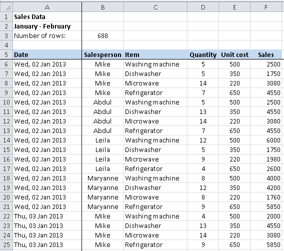
Here's a sample of the sales data we used (note the number of rows - obviously there is a lot more sales data in our report than is shown here):
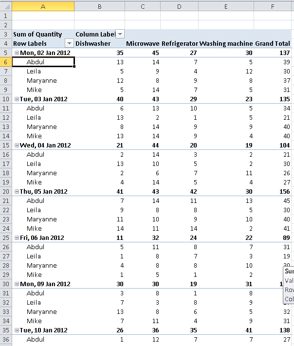
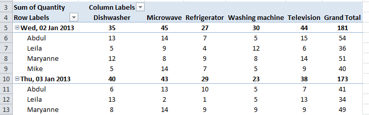
And here's the resulting Pivot Table:
Change the Source Data for your Pivot Table
In order to change the source data for your Pivot Table, you can follow these steps:
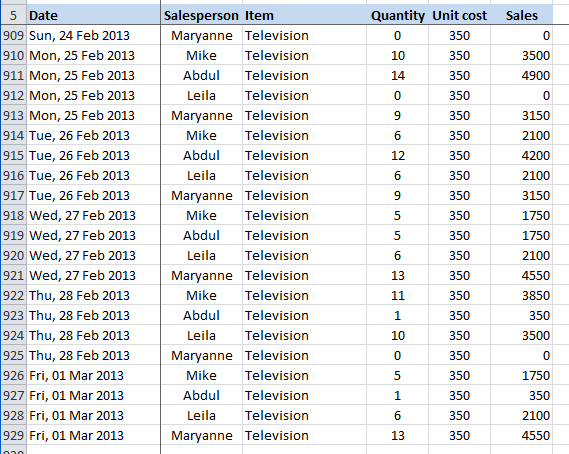
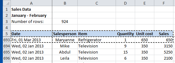
- Add your new data to the existing data table. In our case, we'll simply paste the additional rows of data into the existing sales data table. Here's a shot of some of our additional data. As you can see, we now have 924 rows of data:
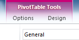
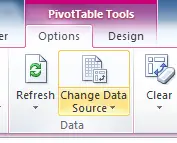
- The next step is to click inside your pivot table so that the Pivot Table tools options appear in the ribbon toolbar, as shown here:
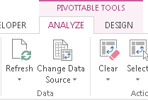
- From there, click Options in Excel 2010 or earlier, or Analyze in Excel 2013. This will show you a range of different options for managing your pivot table. We are interested in just two buttons on this toolbar - the Refresh button and the Change Data Source button:
- It's important to understand what these buttons do, and how they differ:
- The Refresh button will update your pivot table to reflect any changes in your existing data, such as any changes to our sales data due to customer returns. Using the Refresh button won't automatically pick up any new data in your table (unless you're using Excel's Table feature as the source for your pivot table - we'll come to that shortly). Note that you can also choose to refresh your data by right-clicking anywhere in your pivot table and choosing Refresh from the menu.
- The Change Data Source button will allow you specify a new data source for your pivot table. This is the option we want. Note that we're not actually changing to a new data source, we're simply going to update the existing data source to include the new data.
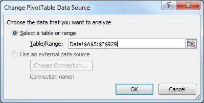
- Click the Change Data Source button to see the following dialog box:
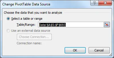
- As you can see, the data range for our existing sales report pivot table is already selected. You can do one of a couple of things here:
- Manually enter the correct data range for your updated data table. In our case, this would mean changing 693 to 929, since the last row of our table has changed from row 693 to row 929.
- Select the new range from the Data worksheet by selecting all the cells you want to include.
- In many cases the second of these two options may be the simplest. The reason is that when you click the Change Data Source button, Excel automatically switches to the worksheet holding the data, and highlights the current data range for you, ready to modify, like this:
(if you're wondering why the rows between 5 and 693 are hidden, it's because this spreadsheet has Freeze Panes turned on, so rows 1-5 are always visible no matter how far down our spreadsheet we scroll. You can learn how to do this in our lesson on how to Freeze or Lock Rows in an Excel worksheet). - The next step is simple: press CTRL+SHIFT together and, whilst still pressing them, press the down arrow on the keyboard. Then release all three keys.
- This uses one of Excel's tricks for quickly selecting large amounts of data (link opens in a new window).
- It keeps the current selection, and extends it by jumping down the spreadsheet to the first blank cell in column A, and stops on the last cell before that.
- Note that this only works if your new data has a value in every row in column A. In our example, we can assume this is the case since the column A holds the date each sale was made.
- Your Change Pivot Table Data Source dialog box will how look like this:
- Assuming the correct data range has been selected, you can now click OK to update your Pivot Table.
- If you get it wrong, and the wrong data range has been selected, don't panic! Simply try again to select the correct range OR click Cancel and start again OR press CTRL + Z to undo the change.
- Here's a sample of our spreadsheet now we've added the Television sales data. Note that we did nothing to the Pivot Table itself - we simply added the new data:
Some points to remember about updating the data in your pivot tables:
- You don't need to sort your data to when updating the pivot table. In our example, we added the Television data to the end of the existing data, and didn't sort by sales date. The pivot table updated just fine.
- You can choose any data range when updating your pivot table. We added new data to the existing table. We could just as easily have created a new data table with all of our data on another worksheet, and changed our pivot table to point at the new data.
- Note that if you do point your pivot table to a new table, your pivot table design may change if the new data table doesn't have the same columns as your original data table. This is where CTRL+Z comes in handy, to undo the change.
- If you're using Excel's Table feature, most of this lesson isn't necessary, since Excel uses the table as the data source, and automatically reflects any changes to the table in the pivot table. However, you will still need to Refresh your pivot table to include the new or changed data in the pivot table.
- Finally, you may have noticed the option to Use an External Data Source. This allows you to use an external database. This is reasonably complicated, and outside the scope of this lesson. Suffice to say that this method generally ensures that your pivot table contains the latest data from your database but, once again, you still need to use the Refresh button to update the pivot table.
If you have any comments on this lesson, or questions about how to update the data in your pivot tables, please feel free to post them in the comments section below.
Our Comment Policy.
We welcome your comments and questions about this lesson. We don't welcome spam. Our readers get a lot of value out of the comments and answers on our lessons and spam hurts that experience. Our spam filter is pretty good at stopping bots from posting spam, and our admins are quick to delete spam that does get through. We know that bots don't read messages like this, but there are people out there who manually post spam. I repeat - we delete all spam, and if we see repeated posts from a given IP address, we'll block the IP address. So don't waste your time, or ours. One other point to note - if you post a link in your comment, it will automatically be deleted.
Comments on this lesson
Pivot Table didn't show all data rows after adding new data
Thanks for this topic. I am able to change Data Source to include new data. However, my pivot table didn't show all data rows (some data at the end are hidden) because the pivot table rows keep the same as before. How or what can I do to see all data rows?
Thanks,
Huilan
Missing pictures of pivot tables
from where you talk about 928 lines all the pivot table pictures are missing - its showing a blue square and your comments only.
Images are back again
Hi Chris
Thanks for your post - sorry - the images have been restored now. It may take up to an hour for cached copies of the page to be updated.
Regards
David
Adding new data to PIVOT TABLE
Hi, I was wondering if you can advice me. I added a new row with data (in the middle of the data), and when I refresh the new data is shown in the pivot table as the last row. Is there any way to force the pivot to keep the position in where I inserted the new data?
Thank you
Hit ratio
Is there a way to add a "hit ratio" column, that would divide one column by another to create a hit ratio percentage??
old pivot should get update automatically with new column and da
When we create pivot table after that if we change data source with completely new columns and data, i want only pivot table to update without manually putting columns in pivot table it should refresh column headers and data.
Results
Hi Guys,
When i added a new column to my data sheet, some of my existing results (one column) has changed, how can this be fixed or how does this happen?
Any help with this is greatly appreciated!
Thanks
I want to add a new sales person to my pivot table
How do I do this?
Is it possible to download the file for the additional data that you are adding to the pivot table in this lesson?