Grouping by Date in an Excel Pivot Table

This lesson shows you how to group data in your pivot table if you have included a date field in the pivot table. This lesson picks up on the work we did in our first lesson on creating a Pivot Table, which introduced Pivot Tables and showed you how to create a basic Pivot Table from a table of source data. In this lesson we will extend that pivot table by grouping our data by date into weeks, months, quarters or years.

In that first lesson, we took a data table that looked like this (note how many rows there are in the table - this table covers a three month period for four sales people):

We then turned that data into a Pivot Table that looked like this:

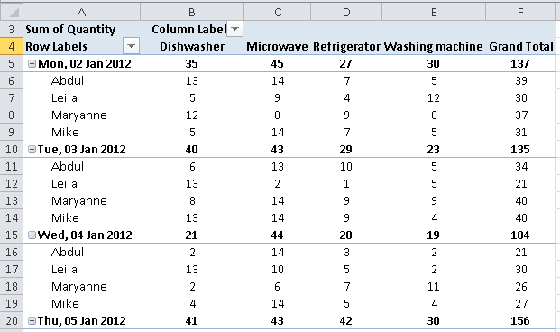
As you can see, the pivot table above has been designed to show product sales broken down first by day and then by sales person. Now, let's look at what else we can do with this pivot table.

We'll start by reviewing how to access the Pivot Table Tools toolbar. This toolbar isn't essential to complete this lesson, but it helps to know how to find it when you need it.

Accessing the Pivot Table Tools toolbar

To access the Pivot Table Tools toolbar, follow these steps:

• Click on a cell anywhere inside your pivot table.
• Check the ribbon toolbar for this option:
  
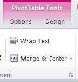
• Then, click either Options or Design to see the related toolbar. The work we'll do in this lesson will focus exclusively on the Options toolbar.

Grouping your data by Date

• To group your data by Date, make sure you have a valid Date field in your pivot table.
  • The Date field in your source data should only include valid dates. If it doesn't, you may not be able to group your data.
  • The Date field can be either a Row or a Column in your Pivot Table, although you may find that placing it in a Row is the most practical option if your source table includes multiple records over a long period of time, since your pivot table will then spread across many columns.
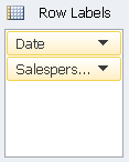
  • You need at least on additional field after the Date field in your pivot table. In our example, our Row fields look like the following. When we group by Date, we will see data for each Salesperson aggregated into the date period that we chose:
    
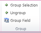
• Once you are ready to group your data, select a date field from within the pivot table and click either the Group Selection button or the Group Field button on the toolbar (both will work in this scenario):
  
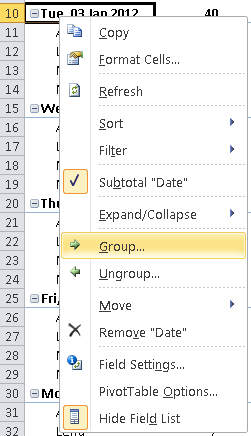
• Alternatively, simply right-click on one of the dates in the first column, and select the Group option as shown here:
  
• Note that if you see a message like this, then either you didn't click the correct date field or some of your dates are not valid date. In the latter case you'll need to review your source data and fix it. Don't bother about clicking the "Was this information helpful?" link unless you want to give Microsoft some feedback on this message.
  
• If you have attempted to group on a valid field type (date in our example), then you will see the following options dialog box where you can choose how you want to group the data in your pivot table:
  
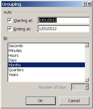
• Excel will automatically select the start and end dates for the grouping based on the dates in your data. You can change these dates at this point so that the grouping only covers a given date range. In our case, we'll leave the dates unchanged.
• You can then choose what you want to group your data by. Note that the Months option has been chosen by default.
• In our scenario, we want to group by Weeks, rather than by Months. As you can see, there is no option to choose weeks. However, we can still get the data to group by weeks.
  • First, click Months to deselect it in the list (Excel will let you group by more than one option, but that's more than we need right now).
  • Then, click Days.
  • Next, enter 7 as the Number of Days value.
  • Finally, click OK.
• Your pivot table should now look something like this:
  
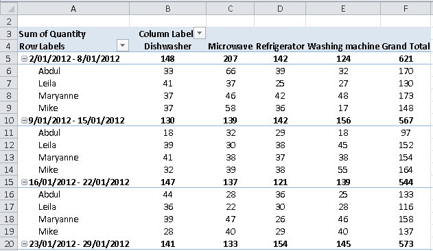
• As you can see in this example, the data has been grouped in 7 day blocks starting from the first date in the data range. If this date was the wrong date on which to start the weekly grouping, (e.g. 2/01/2012 was Wednesday and you wanted the groupings to start on Mondays) then you could repeat the steps above to get to the Grouping options dialog box and change the starting date
• Note that you can remove the grouping at any times by following the steps above and choosing Ungroup instead of Group. The groupings will be removed immediately.

Expanding and Collapsing Data Groupings

Once your data has been grouped, you can then collapse or expand individual group fields to hide the underlying data (in our example, grouping will hide the individual sales people).

• Select the field you want to collapse, and clicking the button to the left of the field heading.
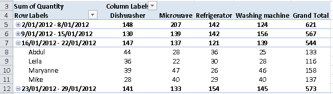
• This screenshot shows the first two weeks collapsed:
  
• You can also collapse or expand all of the fields at once.
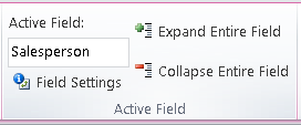
  • Click on one of the fields, and then click either the Expand or Collapse buttons on the Pivot Table toolbar (remember that you need to click on a cell inside the pivot table and then click the Pivot Table Tools button above the main ribbon toolbar).
  • Note that in the example below, the Salesperson field is active. However, it doesn't matter at this point whether the Salesperson or Date field is active - the buttons will do the same thing either way because the Salesperson field is inside the Date grouping.
    
  • If you want more (or faster) control over how you expand or collapse your grouped data, you can also right-click one of the Date fields and choose Expand/Collapse to see different options for expanding or collapsing the fields in the group.
    
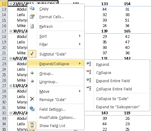
• Let's look at the Expand and Collapse options in more detail:
  • Expand and Collapse will expand or collapse the field you selected. If the group is already expanded or collapsed, choosing those options won't do anything.
  • Expand Entire Field and Collapse Entire Field will either expand or collapse all of the data in the group, i.e. all weeks will be expanded or collapsed.
  • In our example, Collapse to "Date" and Expand to "Salesperson" will have the same effect as Expand and Collapse. This option becomes more useful if you have used more than one grouping in your pivot table.

Summary

This lesson covered two key tasks with Excel Pivot Tables:

• Grouping data based on dates to show your data in aggregated groups (i.e. weekly rather than daily sales data).
• Expanding and collapsing groups to show or hide detail within your pivot table.

As always with subjects as complicated as Pivot Tables, there are more things you can do, and more options to explore. If you've found this lesson useful but want to know more, why not ask a question the Comments section below. You can also let us know if there is anything additional you think we should cover.