Freeze or lock rows and columns in an Excel worksheet
When you are working with a large spreadsheet in Microsoft Excel, it's easy to find yourself scrolling down or across and losing track of where you are. This lesson explains how to freeze rows and columns (officially known as "Freeze Panes") in Excel 2010 for Windows and Excel 2011 for Mac.
Why you might need to freeze rows or columns in your spreadsheet
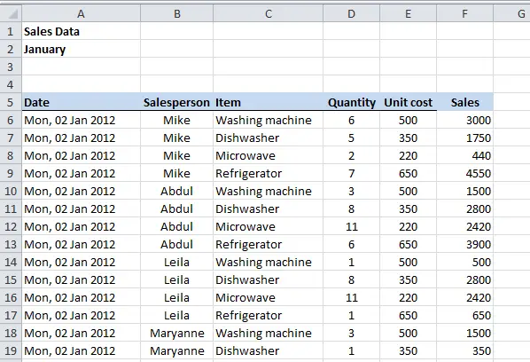
- Imagine you have a spreadsheet that contains sales data for January. The worksheet contains daily data that reports the sales for each person in your sales team, broken down by products sold:

- This example actually has 85 rows of data (the table carries on down further than this screenshot shows):
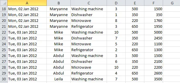
- Once you scroll down, however, the heading row disappears off the top of the screen, and you can no longer be sure what each column contains:

- This is a simple example, but it's not hard to imagine that with a lot more columns and rows, the problem would get considerably more complex,
- To solve the problem, you can freeze or lock the heading rows so that they don't disappear off the top of the screen as you scroll down the worksheet. The proces for doing this is slightly different between Excel 2010 for Windows and Excel 2011 for Mac, so I've covered both here:
How to freeze rows and columns
- You have two options for freezing panes in Excel. Note that these steps also apply to freezing columns:
- Freeze several rows and/or columns
- Freeze just the first row (or column)
- To freeze just one row, click the View menu, and find the Freeze Panes button (if you're using Excel 2011 for Mac, click the Layout menu to find the Freeze Panes button)

- When you click the Freeze Panes button, you can choose Freeze Top Row from the expanded Freeze Panes options. If you wanted to freeze the first column, you would then go back and choose that option. The screenshot below is from Excel 2010 for Windows. In the Mac version of Excel the options are the same, but you don't get the explanations of each option that you see here:

- Things get slightly more complicated if you want to freeze more than one row or column. If you look at the first screenshot in this lesson, you'll see that the first row doesn't actually contain the headings for the sales data table - it contains the title of this worksheet.
- To freeze the heading row of the table, you will have to freeze the first five rows in the worksheet. To do this, click in the cell A6 (i.e the first row that should not be frozen) and choose the first option in the Freeze Panes drop-down menu (it's also called Freeze Panes).
- When you do this, not much will appear to change. All you'll see is a line stretching across the screen, almost like a border along the bottom of row 5 (which is the last row to be frozen in our example). The screenshot shows what Freeze Panes looks like if you had clicked B6 before clicking Freeze Panes (i.e. you wanted rows 1-5 and column A to be frozen):

- Here's what the sales data table looks like if you scroll down. As you can see, the first five rows have stayed put, and the other rows have disappeared underneath them as I've scrolled down the screen:

How to unfreeze panes in Excel
Unfreezing panes is, fortunately, fairly simple:
- In Excel 2010 for Windows, choose the View menu, click the Freeze Panes button. The first option, which was Freeze Panes, is now Unfreeze Panes. Click that option and the frozen rows will be unfrozen.
- In Excel 2011 for Mac, choose the Layout menu and choose Unfreeze Panes (for some reason, it's a separate option which only becomes available once you have frozen panes).
Join our mailing list
Our Comment Policy.
We welcome your comments and questions about this lesson. We don't welcome spam. Our readers get a lot of value out of the comments and answers on our lessons and spam hurts that experience. Our spam filter is pretty good at stopping bots from posting spam, and our admins are quick to delete spam that does get through. We know that bots don't read messages like this, but there are people out there who manually post spam. I repeat - we delete all spam, and if we see repeated posts from a given IP address, we'll block the IP address. So don't waste your time, or ours. One other point to note - if you post a link in your comment, it will automatically be deleted.
Comments on this lesson
Sort a column AND still retain the #1 heading 'row' intact
I use 'Excel for Mac 2011'.
I understand the use of freezing panes.
How do I sort a column AND still retain the #1 heading 'row' intact at the top and not be included in the sort?
NB: I need to globally select the WHOLE column - as I have hundreds and hundreds of rows and I don't want to have to selectively select the data in the column ie by leaving out the heading.
I am unable to get the above solutions working in Excel for Mac.
Solution will be greatly appreciated.
Turn on Autofilter and sort from within there
Hi LR
I know your pain ... I have an Excel spreadsheet that does this to me as well. Not sure if it's a Mac thing, but it's an old Excel for Windows spreadsheet that I transferred to the Mac. Oddly, I don't have that problem if I create a new table in the Mac version.
Three ways to do what you want:
- Enable Autofilter for the table, and then use the Sort option within the Autofilter dropdown on the column you want to sort by.
- Do an Custom Sort and specify that "My list has headers".
- Convert the data to an Excel Table. Click inside the data (make sure Autofilter is off), click the Tables ribbon option, then click the New table button (the first button on the Tables ribbon). This will convert it to a Table and sorting should respect the headers.
I hope that helps!
David
Problem solved - a few other tips for other people
Hello David
Works great - thanks.
(you were a lot more helpful than Microsoft).
A few other tips for other people:
1. Make sure there are no empty cells in the heading row.
2. Make sure heading row consists of only ONE row.
Thanks again
LR
Problem solved + a few other tips for other people
Hello David
Works great - thanks.
(you were a lot more helpful than Microsoft).
A few other tips for other people:
1. Make sure there are no empty cells in the heading row.
2. Make sure heading row consists of only ONE row.
Thanks again
LR
Freezing top row only works in "Normal" view-at least on Mac.
I did not see it mentioned in the lesson and was frustrated when the freeze did not work but I was working in "Page Layout" view and when I switched to "Normal" view it worked just fine. If you freeze the header row in "Normal" view and then try to switch to "Page Layout" view a warning pops up saying that you will lose the freeze.
Works for Excel Mac 2011
Hi, thanks a lot for the detailed steps!
I can confirm these steps will work in Excel for Mac 2011
Just what I needed thanks
I know how disheartening it is when someone reads something useful on a website or blog and then just leaves. So I thought I would take a quick moment and leave a comment letting you know that this is just what I needed to help me with my Excel spreadsheet. Thanks so much for taking the time to post this and share with the internet!
Very Useful
Many Thanks! I've looked for this solution a lot of time! Thanks for your helpful article/lesson.
Regards
Massimo

We are PC users, but sometimes working with data on the MAC is annoying as the commands are different. We looked all around on the web, but this was the easiest way to fix the header / top row issue. Freeze Frames on the MAC is located on the right hand corner and sometimes may be a little small but the icon is exactly the same as pictured above. Thanks FiveMinuteLessons, as you just made the life of one small business much easier.