How to use Excel's INDEX function to find data in a table
Excel's INDEX function allows you to look up a cell contained in a column or table of data in an Excel worksheet, and return the value found in that cell. There are several scenarios where the INDEX function can come in handy when working with Excel. Here are some examples.
- You have a list of values in a column or row, and you want to find out the third value in the list.
- You have a table of data (multiple rows and columns). You want to find the value in the cell located at the junction of the third row and the fifth column in the table.
It's important to note that INDEX can seem somewhat limited when used on its own. For that reason, it is best used in conjunction with other functions such as MATCH or DAY in order to take full advantage of its power.
Excel's INDEX function syntax
Let's look at the INDEX function in use in a simple scenario. First, let's look at the syntax of the INDEX function:
The INDEX function has the following syntax. Note that there are two different versions of the INDEX function, the Array form and the Reference form. We'll be focusing on the Array form in this lesson, but I've included the Reference syntax as well, for completeness.
- =INDEX(array,row_num,[column_num]) - this is the array form of the INDEX function.
- =INDEX(reference, row_num,[column_num],[area_num]) - this is the reference form of the INDEX function.
Note that the use of [] around an argument means that it is optional when you are writing a formula using the INDEX function.
The three elements in the Array form of the INDEX function are as follows:
- array refers to the range of cells you want INDEX to look in, such as A1:A10 or A1:C10.
- row_num refers to which row you want INDEX to look in. This is just a number (although you can use a formula to find the number if you want)
- column_num refers to which column you want INDEX to look in. It's optional and you only need it if you want to look in a column other than the first column in the array you specified.
The four elements in the Reference form of the Index function are as follows:
- reference refers to the range of cells you want INDEX to look in. You can have more than one range of cells, e.g (A1:B10,G1:G10)
- row_num refers to which row you want INDEX to look in, as we saw for the Array form of INDEX.
- column_num refers to which column you want INDEX to look in. It also works the same as in the Array form.
- area_num refers to which reference range you want to look at. If you set reference to (A1:B10,G1:G10), you would set area_num to 2 in order to tell INDEX to look in the second range.
Note that if you only define one range of cells in reference then the Reference form will work exactly the same way as the Array form.
An example of the INDEX function in action
Now let's look at a simple example of the INDEX function in action. As noted above, we are going to concentrate on the Array form of the INDEX function in this lesson.
Imagine you have a spreadsheet that show sales by the day for the last four weeks, and you want to find the sales for Wednesday in the first week. Remember - this is a simple example to illustrate how INDEX works. Your real world examples are likely to be complex than this.
- Here's the spreadsheet with the sales data:
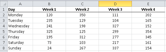
- Note that Wednesday is in the third row of the table (I'm going to ignore the heading row in this example).
- We can write the formula to find the value for Wednesday of Week 1 (241) in several ways:
- =INDEX(B2:B8,3)
- =INDEX(B2:B8,3,1)
- =INDEX(B2:E8,3)
- It's important to note that each of these formulas gives the same result.
- In the first version, Excel assumed column 1.
- In the second version, we explicitly stated it should look in column 1.
- The third version is the same as the first, except we provided a bigger range of cells to look in. That doesn't matter - Excel will still look in the first column unless we specify otherwise.
Now let's get a bit more clever, and find out the sales for Sunday in Week 3
- Note that Sunday is in the seventh row of the table and Week 3 is in the third column.
- We will write the formula in the following way, remembering that we must now specify which column we want to look in.
- =INDEX(B2:D8,7,3)
Summary of the INDEX function
Excel's INDEX function is a powerful function when you want to find a value in a specific row and column location inside a table of data. Our examples used numeric values to identify the row and column values that INDEX should work with. However, you can use other formulas inside the INDEX function, or references to other cells in your worksheet, in order to make INDEX more useful and effective in your Excel spreadsheets.
Do you have a specific example in which you want to use the INDEX function? Why not post a comment describing your scenario, and we'll see if we can add it to our list of examples in this lesson.
Join our mailing list
Our Comment Policy.
We welcome your comments and questions about this lesson. We don't welcome spam. Our readers get a lot of value out of the comments and answers on our lessons and spam hurts that experience. Our spam filter is pretty good at stopping bots from posting spam, and our admins are quick to delete spam that does get through. We know that bots don't read messages like this, but there are people out there who manually post spam. I repeat - we delete all spam, and if we see repeated posts from a given IP address, we'll block the IP address. So don't waste your time, or ours. One other point to note - if you post a link in your comment, it will automatically be deleted.
Comments on this lesson
This might work
Hi Mickie
I was inspired by your question to write a whole new lesson on how to use the INDEX function to return all the values from a list that match the look up value. You'll need to expand on it a little to meet your requirements. Specifically, you'll need to add columns to your Form spreadsheet for every value that you want to include from your Crop worksheet. So if a land owner could have up to 5 parcels, and you want to include 7 values for each parcel in the mail merge letter, you'll need 35 columns with a version of this formula.
I hope that helps!
David
Is this part of the text correct?
Just to comment on the below section of text;
"Now let's get a bit more clever, and find out the sales for Friday in Week 3
•Note that Friday is in the seventh row of the table and Week 3 is in the third column.
•We will write the formula in the following way, remembering that we must now specify which column we want to look in.
◦=INDEX(B2:D8,7,3)"
I cannot understand why you have stated that Friday is the seventh row of the table unless, I've completely misread something here or you mean Sunday?
Surely if your (fx) =INDEX(B2:B8,7,3)
This means,
(row1)B2=Monday,(row2)B3=Tuesday,(row3)B4=Wednesday,(row4)B5=Thursday,(row5)B6=Friday,(row6)B7=Saturday,(row7)B8=Sunday,7(Sunday),3(Array Intersection of row7 vs column 3(column 3 being column D) = 337
Is this correct or can you explain?
KR,
Ollie.
Thanks for spotting the error!
Hi Ollie
Thanks for spotting that. It should have referred to Sunday in the 7th row. I've updated the lesson to fix that mistake.
Regards
David
How to get that row no as per users choice without fixing in for
I have a file with three worksheet. one is invoice sheet other delivery order and third master data. once i put value in master data sheet other two sheet use the same and prepare the invoice and delivery order. Problem is we want to keep the master data updating and get the invoice and delivery order for new rows(new customer detail) on master sheet. i have tried to keep one cell on invoice sheet as reference to the row number the entire sheet can use to get value from master sheet but it doesnt work. How can we get the detail of entire row of master sheet on invoice and delivery sheet by just putting one reference like the serial no of master sheet in invoice sheet
Using Index?
Hi there-
I thought that Index would be the solution to my question, but now I'm not sure as I don't have the exact Row location that I would be looking to return the value from. Here's my situation:
I have a long list of account names, and sometimes they show up multiple times (as we have multiple action items associated with each account), and I want to return a value from some of the Columns associated with the accounts.
For example, the list looks like this:
Account Name/Scheduled Call/Follow-Up/Call Attempt
Account A/Call Complete/(blank)/(blank)
Account B/Call Complete/(blank)/(blank)
Account B/(blank)/(blank)/Attempt
Account B/(blank)/(blank)/Attempt
Account C/(blank)/Follow-up/(blank)
Account D/Call Complete/(blank)/(blank)
Account B/(blank)/Follow-up/(blank)
Account D/(blank)/Follow-up/(blank)
So in this example, a rep completed a call for Account A... and that's the only action item associated with that account. But, for Account B, there are many action items associated with the account: in total they had 1 call, 2 attempts, and 1 follow-up...
In my Summary, I'm trying to do something like a Vlookup, to compare against all our account names, but Return the values as Yes/No of the action items done over a 3 month period. Lookup the account value and return... Yes/No- was a call completed? Yes/No- was there an attempt? Yes/No- was there a follow-up?
Any suggestions on this problem? Please let me know if more details need to be provided! Thank you for your help!!
Kathleen
Try a Pivot Table
Hi Kathleen
I think that a Pivot Table would be better for what you're trying to do (which is quickly summarise a large number of rows of data).
I recreated your spreadsheet and produced the following table using a PivotTable:
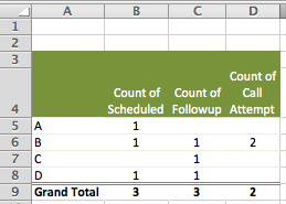
You can read our lessons on Pivot Tables here, although the current lessons don't quite cover everything you'll need to know for this example. I'll be adding a lesson based on your example soon, but here are the key points:
- When you create the Pivot Table, drag and drop the Scheduled, Followup and Call Attempt items into the Values section of the Pivot Table builder.
- Since you have text values in these columns, Excel will default to counting them, yielding the results above.
- This solution assumes that your spreadsheet only has values in the Call Completed, Followup Call and Call Attempt columns where there was some activity, i.e. the other cells really are blank. If they aren't, this solution won't work since Excel will count all of the cells that contain a non-blank value.
Hopefully this gives you a pointer in the right direction. Let me know if it doesn't solve your problem.
Regards
David
Hi David-
Hi David-
Thanks for the quick reply! I think a Pivot Table will work, but my only fear of it was that Pivot Table was going to be my next step... Of the accounts that had calls completed, how many of them renewed? (so I would have to compare the account name, with the won/lost status, etc)
Would I still be able to do another Pivot Table off the Pivot Table example above?
Thanks again!!
Kathleen
Depends on how your data is structured
Hi Kathleen
How is your data set out? Is the won/lost information in the same table as the data for your initial Pivot Table, or in another table?
Regards
David
Help
Gidday
I have a table with about 10x10 which has data numbers in it C3:L13, labelled 1 to 10 on x axis and different number headings on the y axis. Based on numbers calculated in another sheet, i want to write a formula for calling a particular cell within the table. Im a little lost how to go about it.
IE say if my value needed to be in the D column and row 13 based on the calcs, how would I write the formula?
Similarly if I changed my calcs to E and 6 i dont want to have to manually search for it.
Use of INDEX function
In the file attached, I want to search both sets (Set1 & Set2) of numbers, fine and display all the same numbers in the Similar Numbers column.
Copying data from a table in one workbook to a table in another
I have 2 data files (Team Lead Summary 2014 Automation Test.xlsxx and Test-AutoImport.xlsx). Both of these files are stored in the same folder on my desktop. (c:\users\my.name\desktop\myFolder)
In the file Team Lead Summary 2014 Automation Test.xlsx, I have a worksheet called Rep Performance Comparison and a table called WeeklyComparison with 8 columns and 10 rows (my table range is in cells A7:H16).
In the file Test-AutoImport.xlsx, I have a worksheet called Weekly Summary and a table called WeeklyStats with 8 columns and an undetermined number of rows (new data is appended to the table weekly). The table range to start is A16:H17. I also have the username stored in cell B3.
I am trying to Search column 1 (cells A7:A16) in the WeeklyComparison table for a value stored in cell B3 of the Test-AutoImport.xlsx file, and copy the data in columns 2-8 (B7:H7) to columns B17:H17 of the WeeklyStats table.
Here's the formula I am using:
=INDEX('Team Lead Summary 2014 Automation Test.xlsm'!WeeklyComparison[#All],SMALL(IF('Team Lead Summary 2014 Automation Test.xlsm'!WeeklyComparison[#All]=$B$3,ROW($A$8:$A$100)),ROW(17:17))-1,3)
I enter the formula as an array formula (CTRL+SHIFT+ENTER) and get a #N/A error.
Can anyone tell me what I am doing wrong?
P.S. I can only attach one file, so I have included both of the referenced worksheets in my sample file. I've also included my formula as a comment in cell B17 on the Weekly Summary worksheet.
Share rates transfer
Dear Sir,
in my file name has multiple names and values
and i want the value of last rate of name similar to the name 2 in the coloumn D that is rates.
Is there any formula for such.
if yes then please kindly let me know as soon as possible
Is this function for me?
Hi,
Trying to solve problem with spreadie at work.
Have column of alpha-numerical data (e.g. S1002) codes divided by text "shift end".
Is it possible to sort it all in two additional separate columns? Column one all data abowe "shift end", column two, all data below "shift end"?
Cheers!
I.
excel
I have a spreadsheet with dates in horizontal cells and peoples names in vertical cells. At the intersection of the date/name array is further data. Can lookup or other functions be used for finding the data using only date and name inputs and not row numbers?
How to Use Index Match in a table
Hi, I am not very familiar creating formulas or the use of Index Match.
I work in Clinical Research and we note by country, the number of the the CRA would have spent on site. So, In my table I have put in columns to count the number of Days someone spent at a medical site. This can be anywhere from 1 to 4 days. I then must break this information further out by country and days at the bottom of the sheet.
Would it be possible to use Index Match or create a formula that would look at Ukraine, for example, and give me the number of days spent on site ranging from 1 day to 4 days, then give me a '0'. The information is included in the upper part of the table.
Days on Site
Country 1 Day 2 Days 3 days 4 days
Belgium 3 0 1 0
Canada 5 0 0 0
France 9 0 0 0
Germany 3 1 0 1
Korea 5 0 0 0
Russia 5 0 0 0
Spain 18 0 0 0
Taiwan 4 1 0 0
Ukraine 3 0 0 0
USA 9 0 0 1
Total SIVS 64 2 1 2
Total Visit Days 69
Please forgive me if my question takes you in a circle and trust it is comprehensive.
Thx,
D.
How to solve this!
Hi,
suppose I have multiple records for same ID in sheet one.
In sheet two, there are few selected unique Id's from the sheet one.
Now, in sheet three I want all the records from the sheet one for the selected unique ID's in sheet two. Like for eg. consider Id: 88455 from template sheet. Now I want all the records for this ID from sheet one i.e. Audit sheet in sheet three.
Please tell me how to do this.
Would a vlookup work for this
I want to find the SOV Item that goes with the Bill Code.
There is tab with the entire list of SOV Items. I get this list of Bill code and just manually search for the Bill Code number in the SOV Items tab then paste that next to the Bill Code. And do that for 60+ lines.I tried vlookup but it came back with incorrect amounts when I tried to check it. Should I do INDEX or MATCH instead?
Thank you
Index Formula to pull multiple values against Unique No
Hi All,
I am grateful with your complete post on http://fiveminutelessons.com/learn-microsoft-excel/use-index-lookup-mult.... Yesterday I was completely stuck to retrieve multiple values against same number. As vlookup extract only 1st value. By reading and understanding Index formula especially with ISERROR() was awesome. You saved me from doing manual works. I am really grateful with above link and post. Thanks to all who posted and help every one in the world. Thanks Amit
Multiple identical values across several columns - need one
Hi
I have a spreadsheet which collates a number of customer responses to an issue. The repsonses are all held in separate tabs depending on what the subject of the question was.
I have collated this into one sheet so that i can see the full range of response from each person based on their unqiue reference. However, as they are not obliged to answer all questions, I have had to put data from all tabs into the one sheet. This means that I have multiple records of the person's details, the date of the response etc.
What I am looking for is a formula which looks at various cells, some of which are blank and some of which have a value (which will be the same value for all populated cells) and give me that value back. I have already tried a nested IF statement but there are 10 columns of data so it didn't seem to like that.
Any help much appreciated.
how to look up column header and leftmost value
My company gave me a project to make a cable sizing spreadsheet in two months. Now i have gotten to a cross road where i need professional assistance. I am dealing with about 16 tables. and my spreadsheet is designed to make intelligent decisions when the user inputs some random values. From the table i uploaded, my calculation returns 43.5 amps. i need excel to return/suggest an equal or approximate (must be greater) amp available in the tabulated reading. also, i need excel to return the left-most cable size column corresponding to the approximated tabulated amp(returned by excel), and if possible, the column header of the column where the approximated value is found.
Pls, find attached excel sheet titled cable sizing. That should explain my intentions clearly. Kindly give me a detailed solution to this problem. i have exhausted all options i could lay my hands on.
How to pull data from a master into a transaction sheet
I have a prospect master. To call a prospect, I pull the prospect name from the master into the calling record sheet ("Pipeline"), and use VLOOKUP to pull the corresponding phone number and location also from the same record in the master into the calling record sheet.
So, may calling record may look like
1 Anil Kumar 23415016 New Delhi (record no 10 in the prospect master, and the phone number and the location are consecutive cells in the same record)
2 Rashmi Sinha 9811023400 Hyderabad
3 Anil Kumar 9321376938 Mumbai (record no 329 in the prospect master)
When I use VLOOKUP, it picks the first occurrence of Anil Kumar in the prospect master and populates the phone number and location from the first occurrence.
So instead of Anil Kumar 23415016 New Delhi and Anil Kumar 9321376938 Mumbai, I get both as Anil Kumar 23415016 New Delhi.
How do I correct this?
Lookup Table
I am creating a table with equipment down Column one and tools across the top of row one. I need to have my formula first look for the Tractor/equipment used and then the tool/machinery pulled behind that particular implement and come up with the cost per acre in the intersecting cell on the table. After the cost per acre is found I need the formula to multiply it by the number of acres in a cell for that particular field (separate table).
I would also like to look up the owner and return a value of zero so they are not being billed for their own equipment.
Table 1
OWNER Name Name Name Etc.
"No
Implement" Flex Head Protill Air Bougault Air Bougault Salford "Super
Harrow" Wishek Cultivator
Equip
Equipment
Implement
No. of Passes
No of Acres
Total Cost
Table 2 No Implement - Wishek Disk - Chisel Plow
IH Tractor $18.00 25.00
Quad Track $15.00 30.00
Combine $200 0 0
First I need to know what type of tables and also what formulas. It has been ALONG time since I have worked with any of this. I will most like need
if statements, i.e. if cell "X" = Quad Track and Cell "Z" = Wishek Disk, then look up " " on table 2.
I don't know if this is even making sense, I hope so!
Thank you!
Kat R
Lookup or Index
Hi there! I am having trouble figuring out how to extract the information I need in this spreadsheet. Basically, I have a list of qualities (Leadership, Teaching, Knowledge, etc.) and people with those qualities. The spreadsheet has each quality and the people with those qualities, but I need a list of each individual and all their qualities. Is this possible?
Thanks in advance!
Lookup question
Never mind. I figured it out!
Lookup question
Never mind. I figured it out!
Wendy, do tell! What was the
Wendy, do tell! What was the solution?
kshitij.agarwal360@gmail.com
City Mumbai Chennai Banglore Pune Thane
Economy 2100 1900 2000 2100 2050
Mid Range 3300 2900 3100 3200 3150
High End 5100 4700 4900 5000 4950
In case there are two dropdown lists -
1. City ( User can select from Chennai, Banglore, Mumbai, Pune, Thane)
2. Quality ( User can select from Economy, Mid Range, High End)
Is there a way to generate a cell that can take values from the two dropdown selections and produce a result of value from intersecting cells as per the above table?
Working on a project..thanks
Hello,
I'm not sure what function to use in this situation or if it even do-able.
I am using Excel to prepare letters that go to landowners whose crops were affected by recent construction. I am using a template for a mail merge to print letters to the landowners that is working beautifully. However, I want to be able to pull the information about that landowner's crops from another worksheet onto the letter. If it was a one-to-one reference, it wouldn't be a difficult task.
However, some of the landowners have several parcels of land. This has been entered into the spreadsheet using an individual ID number that was used during construction. Example:
ID No. Name Crop Twp Rng Sec
H240 John Smith Soybeans 1N 14E 12
H240 John Smith Corn 1N 14E 11
H240 John Smith Corn 1N 15E 9
W569 Amy Nelson Soybeans 2N 12E 2
There are many more columns in my table that have the formulas used for calculating the offer based on type of crop, county, length, yield, etc.
My question is how can I pull the rows of information for each landowner's crops from the "Crop" worksheet onto the "Form" worksheet? When I print the letter for John Smith his three parcels of land will appear on his letter and Amy Nelson's parcel will appear on her letter, etc.
Respectfully,
Mickie