How to use INDEX MATCH instead of VLOOKUP
This lesson shows you how to write formulas using INDEX and MATCH to let you perform lookups that VLOOKUP can't, and which run much faster on large spreadsheets than VLOOKUP. This lesson explains how INDEX and MATCH work on their own, and then shows you how to write an INDEX MATCH formula that can look left as well as right, and performs much faster than VLOOKUP on large tables.
INDEX MATCH works very well if your lookup data is not in the first column, or you want to look to the left of the lookup data, rather than to the right (which is all VLOOKUP can do).
Note - Microsoft have announced a new function, XLOOKUP, which does the same job as the INDEX/MATCH workaround described in this lesson. It's in beta right now, and is only available on Office365. You can read more about how to use XLOOKUP here.
What you'll learn in this lesson
In this tutorial, you'll learn:
- How to use the MATCH function
- How to use the INDEX function
- Scenarios where VLOOKUP doesn't work or isn't the best solution.
- How to combine the INDEX and MATCH functions in your formulas to perform lookups that VLOOKUP can't.
Why INDEX MATCH is so much better than VLOOKUP?
For many users, VLOOKUP just does what they need. But there are three scenarios where VLOOKUP falls short. That's where INDEX MATCH comes in handy:
- VLOOKUP can only look from left to right.
- You look a value in one column in a table, and then return a value from a column to the right.
- But what happens if you want to look from right to left? VLOOKUP simply can't do that. INDEX/MATCH can.
- VLOOKUP is prone to error, especially in big spreadsheets
- With VLOOKUP, you specify a number to represent which column you want to return the value from. So you have count the columns to figure out which one you want. Hopefully you'll notice if you get it wrong but what if you don't? Finding and debugging this error can be a nightmare.
- With INDEX MATCH, you select the specific column of data from which you want to return the value. That's much more reliable and easier to debug when things go wrong.
- VLOOKUP slows down big spreadsheets.
- When the value you are looking up is in one column, and the value you want to return is in the 30th column in the table, VLOOKUP requires you to select all 30 columns. This results in a lot of extra computations and can bring large spreadsheets to their knees.
- With INDEX/MATCH, you select the column containing the lookup value and the column containing the return value, and nothing else. That makes INDEX/MATCH much more efficient.
Recap of what the INDEX function does.
The INDEX function has a very simple job - look in a column of data and return a value from the row that you specify.
Here's an example of the INDEX function in action:
=INDEX(A2:A8,3)
In this example, we tell Excel to return the 3rd value in the range A2:A20. Here's what that looks like:
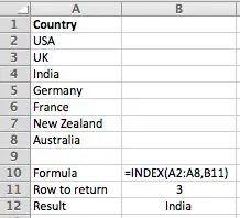
Note that I've changed the formula from above to use the value in B11 as the row to return, rather than typing 3 directly into the INDEX function.
You can read more about the INDEX function in these lessons: How to use the INDEX function to find data in an Excel table and Use INDEX to lookup multiple values in a list. Both links open in a new tab.
Recap of what the MATCH function does
The MATCH function also has a simple job - look in a column of data and return the row number of a value that you specify. It's a bit more complicated than the INDEX function, but we'll use it in a simple way in this lesson. You can find out more about the MATCH function in this lesson: Use the MATCH function in Excel to find the position of a value in a list (opens in a new tab).
Here's an example of the MATCH function in action. Let's assume we have a column of names, and we want to know which row Birgit is found in. We'll assume that each name appears only once in the list - this will make things simple for us.
=MATCH("Birgit",B2:B8,0)
Here's a worked example to illustrate the use of the MATCH function:
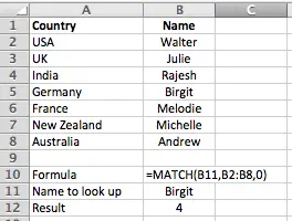
As you'll see, I've adjusted the example to use the value in B11 as the value to look up, rather than typing "Birgit" directly into the formula.
Note that the third parameter in the formula is the match_type. By entering zero as the last parameter in the formula, we tell Excel we are looking for an exact match. The VLOOKUP function has a similar parameter, but the MATCH function uses this parameter differently. I won't go into the differences here, but if you're planning to use the MATCH function a lot, you should read our lesson on how to Use the MATCH function in Excel to find the position of a value in a list which covers the match_type parameter in detail.
Putting INDEX and MATCH together
Now that we understand what the INDEX and MATCH functions do on their own, let's put them together to create an INDEX MATCH formula that can replace VLOOKUP - and do much more..
Example 1 - Use INDEX MATCH to replace VLOOKUP
Let's start with a simple example, and use INDEX/MATCH to do something that VLOOKUP can do - find the name of the person from France.
First, here's the VLOOKUP function you would use to do this:
=VLOOKUP("France",A2:B8,2,0)
This formula says "Look for France in column A and if you find it, return the value from the second column in the same row. If you don't find France, return an error"
Here's how we can do this with INDEX/MATCH:
=INDEX(B2:B8,MATCH("France",A2:A8,0))
This formula says "Find the row that contains France in column A, and then get the value in that row in column B. If you don't find France, then return an error".
Here's our example with this formula combining INDEX and MATCH:
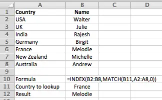
Once again, note that I'm using B11 in my formula rather than typing "France" directly into the formula.
Example 2 - Using INDEX MATCH to look from right to left.
Obviously, when compared to the VLOOKUP version of the formula in the example above, using INDEX MATCH results in a longer formula. For that reason, you may prefer to keep using VLOOKUP rather than INDEX/MATCH for simple examples.
However, what if we want to do a lookup from right to left, instead of left to right? For example, what if we know the person's name, but want to find out what country they are from?
Let's now look at how we can use INDEX MATCH to do a lookup from right to left, and find out the country a person is from.
Here's an updated version of the previous example:
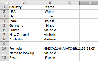
Unsurprisingly, the formula is almost unchanged. We're still finding an item in a list (Melodie) and then retrieving the value in the same row from another column (France).
Why INDEX MATCH is faster than VLOOKUP
At the start, I stated that INDEX MATCH is faster than VLOOKUP.
The reason this is so isn't immediately obvious with the simple examples provided here. However, consider this scenario:
- Our INDEX MATCH formula in Example 1 looks like this:
- =INDEX(B2:B8,MATCH("France",A2:A8,0))
- As you can see, this formula specifies the lookup column (A2:A8) and the value column (B2:B8), whereas the VLOOKUP function doesn't explicitly specify the value column - it simply gives a number that defines where the value column is relative to the lookup column:
- =VLOOKUP("France",A2:B8,2,0)
- But what if our value column were in row AX (column 50) ? Here is how our two formulas would look:
- =VLOOKUP("France",A2:B2,50)
- =INDEX(AX2:AX8,MATCH("France",A2:A8,0))
- Our VLOOKUP formula is going to have to count across 50 columns to find the lookup value - this is going to take time, particularly if you have a spreadsheet with hundreds or thousands of rows, each containing this VLOOKUP formula. If you've worked with a spreadsheet like that you'll be aware that it can take several seconds to recalculate the spreadsheet.
- By comparison, our INDEX function already knows where it needs to look, so it is able to complete its task a lot faster than VLOOKUP. This is good for your productivity since you don't have to wait for the recalculation each time you change a value in the spreadsheet.
- Add to that the fact that our INDEX function is much easier to understand by looking at it - and troubleshoot - than the VLOOKUP formula, and you'll see that INDEX MATCH is also less prone to errors.
Summary - using INDEX MATCH as an alternative to VLOOKUP
In this lesson, we've learnt why VLOOKUP isn't always the best choice when trying to find values in a table based on a lookup value.
- We've looked at an example where INDEX MATCH can do something VLOOKUP can't do (look to the left in a table as well as the right).
- We also talked about how much more efficient and less error-prone the INDEX MATCH combination can be compared to VLOOKUP.
Hopefully this lesson has helped you understand how to combine the INDEX MATCH functions. If you have any feedback on this lesson, or specific questions in relation to the use of INDEX MATCH, feel free ask them in the comments below.
Our Comment Policy.
We welcome your comments and questions about this lesson. We don't welcome spam. Our readers get a lot of value out of the comments and answers on our lessons and spam hurts that experience. Our spam filter is pretty good at stopping bots from posting spam, and our admins are quick to delete spam that does get through. We know that bots don't read messages like this, but there are people out there who manually post spam. I repeat - we delete all spam, and if we see repeated posts from a given IP address, we'll block the IP address. So don't waste your time, or ours.
Comments on this lesson
Multiple ifs
Multiple ifs
Submitted by adicegrani on Mon, 01/05/2015 - 06:43
I am trying a formula with nested ifs.
My formula works perfectly until a number of 64ifs.
Now, I have more problems than 64. How can I avoid them?
PLS FIND ATTACHED A COPY THAT I AM TRYING TO AVOID.
HOPE YOU COULD HELP ME IN THE ISSUE.
Hi,
Excel 2003 has a limit of 7 nested IF's
Excel 2007 has a limit of 64 nested IF's
Mike
mistake in your writing
You wrote, "what if we want to do a lookup from left to right, instead of right to left".
You meant, "(...) from right to left, instead of left to right."
What you are doing here is CALLED 'right to left'. That's the difference from VLOOKUP.
Thanks for the correction
Thanks for pointing that out - I've now fixed the error. Sorry about that!
Regards
David
Anyway to automatically find column number?
Thanks for the post. Correct that index match allows us to look from right to left--that's useful as Vlookup can't do it.
My follow up question is index match helps us find out the row number so we can match the value, but I still have to change the column number manually, is there anyway to make that automatic as well?
Defining column number using a formula
Hi Bingying
It depends on how you want to determine which column to choose.
In the following example, I've written a formula that will look at the value in C12 (City), find the column which contains "City" in the first row, and then modify the INDEX/MATCH formula to look in that column.
Here's the formula so you can copy it and paste it into your own spreadsheet. I've also updated the worked example spreadsheet in this lesson for you to download.
=INDEX(INDIRECT(ADDRESS(ROW(A2),MATCH(C12,A1:C1),4)&":"&ADDRESS(ROW(A8),MATCH(C12,A1:C1),4)),MATCH(C11,C2:C8,0))

The formula does several things differently to the other examples in this lesson:
- Takes the value in C12 and finds it in the column headings (A1:C1) using the MATCH function.
- It has to do this twice to find the start and end of the range that the INDEX function will look in.
- Constructs the cell range for that column.
- In this example, with City in C12, the cell range will be B2:B8.
- Note that the formula uses row 2 and row 8 for the lookup range - this is hard coded so you'd need to modify it for your own spreadsheets.
- The value "4", which appears twice in the formula, is used to define the range using relative references (B2:B8) rather than absolute or mixed references (e.g. $B$2:$B$8).
- Uses the INDIRECT function to turn the cell range (B2:B8) from a text string into an actual cell range that Excel can use.
Note that the formula returns an error if C12 is blank.
You could modify this approach to specify the column number directly rather than using the MATCH function to find the column which contains the value in C12.
Here's a version of the formula that would work if C12 contained the column number rather than the column heading:
=INDEX(INDIRECT(ADDRESS(ROW(A2),C12,4)&":"&ADDRESS(ROW(A8),C12,4)),MATCH(C11,C2:C8,0))
You could then use any method you like to decide which column number to use in the main INDEX/MATCH formula.
I hope that helps.
Regards
David
Index Match Formula
I have a text list from B12-B132
I have a calculated list of numbers in cells g12-g132
In Cell F5 I have a numerical search
And In cell G8 I have this formula
{=INDEX(G12:G132,MATCH(MIN(ABS(G12:G132-$F$5)),ABS(G12:G132-$F$5),0))}
So when I enter a number in cell C5 , G8 returns the closest match.
and highlights the corresponding cell in the range from G12 to G132
What I am trying to do is put a formula into cell E8 which returns the corresponding text.
from B12-B132
Thanks in advance for your help.
Rgds Steve
Vlookup to Index and match
I have a file where I put a lookup table in another tab, I have tried to use the index & match however it keeps coming back to zero. I currently have a vlookup in that field and am trying to make the switch but it is not working.
Here is my index formula =INDEX(A3:A86,MATCH(B3,LKUP!C:D,0)) My current vlookup formula =VLOOKUP(A4,LKUP!C:E,3,FALSE)
your thoughts would be greatly appreciated
Check that your MATCH function is working
Hi Juli
Comparing your VLOOKUP formula and INDEX/MATCH functions, it looks like they are doing completely different things.
- The lookup value in your VLOOKUP function is A4, whereas it is B3 in your INDEX/MATCH function.
- Your VLOOKUP function looks for a matching value in column C. The INDEX/MATCH function looks in the range A3:A86.
- Your MATCH function is trying to look in more than one column. MATCH can only look at one column.
Here's the INDEX/MATCH equivalent of your VLOOKUP function:
VLOOKUP: =VLOOKUP(A4,LKUP!C:E,3,FALSE)
INDEX/MATCH equivalent: =INDEX(LKUP!C:C,MATCH(A4,LKUP!E:E,0))
One further comment is that I would be wary of using whole column references (E:E, C:C) when writing an INDEX/MATCH formula.
The reason is that there are more than a million rows in an Excel worksheet, and MATCH will return the row number of the first row that contains a matching value. However, you've told Excel to take the result of the match function and look in the range A3:A86. If the row number where the lookup value was found is not between 3 and 86, your INDEX function will cause an error.
I hope this helps
Regards
David
Using index, match and large functions
I was trying to rank the students and listing out the names of toppers. I used the three functions index, match and large,1 large2 and so on. The problems occurs when there is a tie between two students. It returns the value that occurs first and does not get the next name. You can find the name of Viki Malhotra repeated twice and the name of Nagesh Majhi does not appear. Can anyone help out tracking out a modification to the formula I have used???
Not sure where to go on this one..Vlookup is the best i can see
Is there any way to search a spreadsheet for location of a word and then set the lookup range based on the location of that word? I have a spreadsheet with Multiple Department Categories and the same sub-category within each main category ( example below and spreadsheet attached). Every day I must generate this report and pull out only some of the data. Each day, the report is a little different, things are never in the exact same row since each day's activity is a little different. Some days, the range of cells underneath each main Dept. category are bigger than other days. I am using vlookup and it is only accurate some of the time since the lookup ranges keep changing and sometimes it returns a number from the wrong Department Category since it is only looking for the sub-category name.
I need to get this (department names and dollar amounts are in 2nd column):
Department Name: WELLNESS
Cashier Negative Report
All Voids $ 199.14
Line Item Discount Report
BOARD 15% $ 8.10
DO 5% $ 4.83
LINE DRIVE 20% OFF $ 63.40
SENIOR 5% $ 12.61
STAFF 15% $ 17.52
Item Discount Totals $ 106.46
Subtotal Discount Report
OWNER 10% $ 178.84
WELLNESS 10% OFF $ 193.30
Subtotal Discount Totals $ 372.14
Combo Discount Report
WELLNESS 10% DISCOUN ($ 0.82)
Combo Discount Totals ($ 0.82)
Sales Totals Report
Department Name: SPECIALTIES
Cashier Negative Report
All Voids $ 58.95
Line Item Discount Report
BOARD 15% $ 1.96
DO 5% $ 1.10
SENIOR 5% $ 1.07
STAFF 15% $ 9.64
Item Discount Totals $ 13.77
Subtotal Discount Report
OWNER 10% $ 29.93
Subtotal Discount Totals $ 29.93
Sales Totals Report
to this:
WELLNESS
BOARD 15% 8.10
DO 5% 4.83
SENIOR 5% 12.61
STAFF 15% 17.52
OWNER 10% 178.84
SPECIALTIES
BOARD 15% 1.96
DO 5% 1.10
SENIOR 5% 1.07
STAFF 15% 9.64
OWNER 10% 29.93
I would love to hear from anyone who can help. I hope my Excel-ese makes sense!
Have you tried a Pivot Table to solve this?
Hi Betsy
It sounds to me like a Pivot Table would do most of what you need. You would need your spreadsheet organised so that your data was in three columns:
Department, Category, Value (although the sequence of the categories won't matter)
You would need to make sure there was a value in every cell in every row (or that you at least have a value in every row for Department and Category).
You can learn how to use Pivot Tables by reading our lesson here. That lesson covers most of what you need to know to solve the problem as I've described.
Let me know if that helps, and feel free to post back here (or in the comments for the Pivot Table lesson) if you still need help.
Regards
David
Index, match and small
Hi, many thanks for the index and match tutorial its been a great help to me. I am struggling with another problem now and was wondering if you had any ideas?
I have a table with 3 columns, colour, cost and code
I want to enter a colour into a cell and then return a list of the 10 lowest costs and corresponding codes for that colour.
I was thinking this could be done with a combo of index,match and small commands but I can't work it out.
My sheet is attached, thanks in advance for any help.
Dan
I
Index Match not working beyond 99 rows
I am using =INDEX('Sr no sts'!C:C,MATCH(A100,A:A,0))
which is =INDEX ( Target Range , MATCH ( Criteria value , Criteria Range , 0 ))
Above formula gives result upto 99 rows but when the same is used in 100th row, gives result as o (zero).
Pl help and let me know what am I doing wrong. I was using vlookup successfully but thought to use index match to reduce calculation time. I am going to use it in more then 9000 cells.
Regards,
Ketan
Pl help.
Pl help.
VLOOKUP slows down big spreadsheets.. but so does INDEX MATCH
Good article, however, it would not be good to confuse that VLOOKUP is slower significantly than INDEX MATCH. In fact 2 TRUE VLOOKUPs will be muuuuch faster than any INDEX MATCH. Apart from than I agree with the other pros of using INDEX MATCH
For my perspective on VLOOKUP vs INDEX MATCH performance feel free to read:
http://www.analystcave.com/excel-vlookup-vs-index-match-vs-sql-performance/
last vlookup example has error
your last vlookup example has an error in it:
"=VLOOKUP("France",A2:B2,50)"
...should be...
"=VLOOKUP("France",A2:AX8,50)"
INDEX MATCH with to linked EXCEL files
I have 2 EXCEL files : the one included in my comment and a second one (CLI.XLSX) containing 2 columns : cli_id, cip
I need to update the cli_id column of the CA.XLSX file thanks to the cip column which is common to both files (value contained in this column is unique).
My efforts to introduce the link method into the INDEX MATCH formula are unsuccessfull !
An example of formula into cli_id of CA.XLSX would be appreciated !
Thank you in advance for your help.
matching problem
i have an excel sheet with five colums one serial number, name, start date, qaulity and qauntity. ou of these i ma supposed to calculate the best qauality and match it with its coresponding name , start date and qauntity, but i have failed. i have just calculated qaulity, and got the correct name but failed to get/or match it with the correct start date and qauntity. pliz help thanks
INDEX MATCH
WITH VLOOKUP, TO RETURN THE VALUE FOR A MONTH, I USE A RANGE FOR THE MONTH (01/01/2016 => 01/31/2016 - 2 COLUMNS). HOW DO I USE 2 COLUMNS FOR THE MATCH IN INDEX MATCH. FOR EXAMPLE, HERE IS MY TABLE. WHEN I SHOW A DATE OF 01/02/2016, I EXPECT A RETURN OF 1. THIS IS NOT WORKING FOR INDEX MATCH. WHAT DO I NEED TO DO? OR DOES INDEX MATCH NOT DEAL WITH MORE THAN ONE COLUMN IN THE MATCH?
Date Date Month
01/01/2016 01/31/2016 1
02/01/2016 02/29/2016 2
03/01/2016 03/31/2016 3
04/01/2016 04/30/2016 4
05/01/2016 05/31/2016 5
06/01/2016 06/30/2016 6
07/01/2016 07/31/2016 7
08/01/2016 08/31/2016 8
09/01/2016 09/30/2016 9
10/01/2016 10/31/2016 10
11/01/2016 11/30/2016 11
12/01/2016 12/31/2016 12
SO TO RETURN 1 FOR JANUARY I WOULD USE FORMULA =IF(A43="","",VLOOKUP(A43,ARGUMENTS!$B$4:$D$15,3))
index + match
Good evening, I am trying to make an excel document where my Marines can enter in their rank and years of service. Once they do this a formula will be able to auto search a column Q1:AQ1 (rank) against a row P2:P23 (years in service) once it matches them it will search an a field for their pay amount (think a times table chart).
My current formula of (below) is coming up as #REF!
=INDEX(Q2:AQ23,MATCH(A2,Q1:AQ1,FALSE),MATCH(A4,P2:P23,FALSE))
The end result will be an auto calculation for the new DOD retirement.
Any help would be greatly appreciated.
I know this is nearly a year old but...
I think this could help: https://www.deskbright.com/excel/index-match-multiple-criteria/
struggling to apply the Index-Match formula
Hi Team
I am struggling to apply the Index-Match formula when pulling the data from other sheet. I want to pull the value to Sheet1 from Sheet2. Can you help with this? Attached is the work sheet and error screen shot.
Index + Match to return any data from specific cells
Below is a formula i have, but needed Excel to return data where, once it finds a match in the index C2 through C132, and matches it with C699, it should return whatever value is in the adjacent cell, which is a range from B2 through B132
=INDEX($C$2:$C$132,MATCH(C699,$B$2:$B$132,0))
any help would be greatly appreciated.
Thanks in advance.
Help needed
Please help me to put the formulae in the attached sheet(activity)Sheet1. What i want is the formula to return the values in the Start and finish columns as typed manually(highlighted). It will be highly appreciated. Thank you
Index & Match
Great Article! Well done!
Using SUMIF in a check register
Hello,
I am currently using excel to keep track of my financial records. It's the end of the year and I'm getting ready for taxes. I would like to take all of my information from the spreadsheet containing my check register, and put it into another sheet that will break down my income and expenses by their designated categories and by whom the transaction was made with. I have uploaded the file I am working on to this comment. Is there a formula or multiple formulas that I can use for this task? This is the formula that I tried to use to add all of the corresponding cell contents together from payments made to Mile Saver Shopper. =SUMIF('Check Register'!'Check Register'!$H4:$L740,'Total Spending'!$B10,'Check Register'!$K:$L) and it did not work. Obviously wasn't correct.
Thanks for any help!
Adding a matched value to Sheet A from Sheet B
How do I add a value from one sheet to another?
Sheet A has a large database, and one of the categories have no phone numbers. Sheet B had that category with the phone numbers. I want to get the phone number that matches the company inserted eg ABC co in Sheet B has phone number 1234, we want to find ABC co in Sheet A, and add the phone number to that line, so in Sheet A, ABC co now shows the phone number 1234
What is the formula to do this?
Need Help In My Excel Project
I need some help that i had been working my excel project very long time but still cant figure out how to complete it. I stuck out in the vlookup in price list sheet. i wanna use lookup to find the product weight shipping cost. But dont know how. can someone help me to solve this problem. I had upload my excel project too. Kindly need someone to help me out.
Hi everyone. I need to help
Hello. I am ltonser. And i need to help. hmmm
Thanks
Thanks good explanation with example, got references from Google and links
Vlookup in multiple columns
My friend came to me with a query and I am trying to find the best way to help:
She has one spreadsheet with 858 rows of HR data and another spreadsheet with 456 updates of data.
She wants to be able to update the Master spreadsheet with the 456 rows of data and not impact the 400 unchanged rows.
What would be the best way to tackle this?
Any ideas welcomed :) She is required to data validate this so we want to ensure anything that is updated / overwritten is clear.
Kind regards,
Edel
I am trying a formula with nested ifs.
My formula works perfectly until a number of 64ifs.
Now, I have more problems than 64. How can I avoid them?
PLS FIND ATTACHED A COPY THAT I AM TRYING TO AVOID.
HOPE YOU COULD HELP ME IN THE ISSUE.