Using SUMIF to add up cells in Excel that meet certain criteria
The SUM function in Excel allows you to add up the values in a range of cells. However, sometimes you only want to add up the cells that meet certain criteria. That's where the SUMIF function comes in handy, along with the more capable SUMIFS function.
There are two common scenarios for using SUMIF:
- You want to add up all the cells in a range that meet a certain criteria, e.g. all cells in a range (e.g. Sales) that contain a value of $500 or higher.
- You want to add up all the cells in a range where the cells in another range meet a certain criteria, e.g. add up all cells in a column (e.g. Sales) where the cells in another column (e.g. Quantity Sold) is 5 or more.
SUMIF function syntax
The SUMIF function has the following syntax:
=SUMIF(range,criteria,sum_range)
- range is the range of cells you want to add up. It is required for the function to work.
- criteria is the criteria which must be met for a cell to be included in the total. It is also required.
- sum_range is the range of cells that will be added up. It is optional; if you leave it out, Excel will check the criteria against the sum_range. In the two examples above, the first example doesn't need you to provide a sum_range, while the second example does.
One of the tricky things when constructing a SUMIF function is how to present the criteria. Here are some examples to help you:
- To add up all values that equal 500: enter 500 as the criteria. Excel knows you want to match cells with a value of 500.
- To add up all values that are greater than 500: enter ">500" as the criteria. Notice the use of quotation marks around the criteria. You'll get an error if you leave those out.
- To add up all values that are greater than or equal to 500: enter ">=500".
SUMIF in action - adding up all sales that are greater than a certain number.
The following example is a simple way to demonstrate SUMIF in action where we won't include the criteria_range argument. We'll use the first scenario given at the beginning of this lesson.
- Imagine you have a table showing sales for the week.
- You want to find the total of sales for only those days where sales were greater than $500.
- You enter the SUMIF formula in to a cell at the bottom of the column of sales figures (along with the SUM formula to give you the overall total)
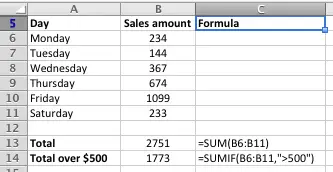
- Row 14 contains the SUMIF function, and the outcome of the SUMIF function in C14.
SUMIF in action - adding up all sales where the sales quantity is greater than a certain number.
Let's extend the example in the table above to only add up sales where the quantity sold was 5 or more. This is the second scenario described at the start of the lesson.
- After adding a Quantity column, the table above now looks like this:
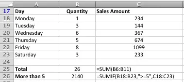
- The formula in C4 has been changed to reflect the new criteria, and has also included the sum_range. Now, the SUMIF function checks the quantities in column B to see if they match the criteria supplied, and adds the sales value in column C if they do.
SUMIF where the criteria are text values
You can use SUMIF to add up one column where the value in another column matches a text value in another column. This might be useful in the previous example where we wanted to add up all rows where the Day column included "Monday". There is an example of how to do this in the comments below.
When using text criteria, you can also use the * as a wildcard to match only a portion of the text value. There is an example of how do to this in the comments below.
SUMIF where the criteria is in another cell
You can also use a cell reference as your criteria (i.e. the value in another cell) rather than a number as shown in the examples above. Let's assume that cell D5 contains the value we want to use for our criteria. Here are a couple of examples of formulas using D5:
- =SUMIF(B18:B23,D5,C18:C23) - this will use the value in D5 as the criteria, and sum any values that equal the value in D5
- =SUMIF(B18:B23,>D5,C18:C23) - this will NOT work, and Excel will not accept this formula if you type it in.
- =SUMIF(B18:B23,">"&D5,C18:C23) - this will use >D5 as the criteria, i.e. any values greater than the value in D5.
- =SUMIF(B18:B23,">="&D5,C18:C23) - this will use >=D5 as the criteria, i.e. any values greater than or equal to the value in D5.
In the third and fourth examples, we have to play a bit of a trick on Excel to get it to recognise our criteria (remember that the second example doesn't work, which is where most people get stuck).
Because we want to combine text (>) with a cell reference (D5) to get our criteria, we have to join them together into a single string of text, which Excel can then understand. This is called concatenation, which you can learn more about here. That's what you'll see in action in the third and fourth example.
Extending the SUMIF function
The SUMIF function is very useful, but has some limitations. For example:
- What if you only wanted to add up sales amounts where the quantity was 5 or more AND the sales amount was greater than $500? SUMIF won't do the job - you'll need to use SUMIFS for that, which allows you to provide multiple sets of criteria and criteria ranges.
- What if the Sales column was actually a Unit price, and you wanted to add up the total sales. You'd need to multiply the quantity by the sales amount, and then find the total. That's where the SUMPRODUCT() function comes in.
What do you think?
I'd love to hear your feedback about this lesson. Did it help? Is it accurate? Do you have a particular problem you want to solve and you can't quite get the SUMIF function to work for you? Why not add a comment or ask a question about your specific scenario below.
Our Comment Policy.
We welcome your comments and questions about this lesson. We don't welcome spam. Our readers get a lot of value out of the comments and answers on our lessons and spam hurts that experience. Our spam filter is pretty good at stopping bots from posting spam, and our admins are quick to delete spam that does get through. We know that bots don't read messages like this, but there are people out there who manually post spam. I repeat - we delete all spam, and if we see repeated posts from a given IP address, we'll block the IP address. So don't waste your time, or ours. One other point to note - if you post a link in your comment, it will automatically be deleted.
Comments on this lesson
sumif maybe
I have a spreadsheet with columns I Actual year to date, j budget year to date and 12 columns M to X with each months budget
Is there a way I can fill column j with the sum of correct rows ie m period 1, m and n period2, m,n,o period 3 etc
I had thought of adding a month no at the top of each column so that if col j row1 had 2 then col j row 5 would add m5+n5 row 6 would add m6+n6 and then increase as i change the month no at the top of row j
Any easy way to do this ???
Thanks
Ricky
sumif function
i want to use sumif function, where i use specific text as criteria in criteria range .
example: use "13ccl01" as criteria
in criteria range cell
CRITERIA RANGE SUM range
13ccl01f01 345
13ccl01f02 234
13ccl01fo3 234
13ccl02f01 345
13ccl02f02 43
13ccl03f01 14
if it is not possible by sumif, then give me another solution
SUMIF using text criteria and wildcards
Hi Sajib
This is actually pretty easy to do using * as a wildcard in your criteria:
=SUMIF(CRITERIA_RANGE,"*12ccl01*",SUM_RANGE)
Here's a picture:

Sumifs with contains
=SUMIFS(H$12:H$101,$F$12:$F$101,$F118)
H-range is the column to sum
F-range is the column to check criteria in (and may contain mulitiple values ie: a, b, c, etc)
F118 is the cell reference to the actual single value for criteria (ie: a)
so I want to sum up all value in H-range if F-range contains F118
Can that be done?
Sumifs with contains
I should clarify that F-Range (in each cell of range) contains multiple values...so the contains on F118 would be to target each cell in F-range.
Sumif( with a cell reference containing text for criteria - See
I am not sure if this is correct way to ask a question, but my question is can I use a cell reference containing text as the criteria in a sumif( function
ie sumif(range.....,B5,range......)
Where B5 may be "Mary" and where there are multiple entries of Mary and I wish to sum the values next to her name
If not a proper way to ask advise, please accept my appology
Yes, you can do this in Excel
Hi
First of all, this is exactly the right place to ask a question. Happy to help!
In answer to your main question, yes you can do what you're asking. By putting your criteria value into a cell, you can then reference that cell when you write your SUMIF formula.
I've created a simple example to illustrate how this might work.
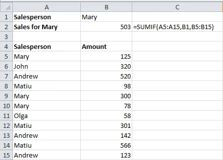
I've included column C in the picture because it includes a copy of the formula I used in cell B2.
Essentially, this formula references cell B1 to find the criteria for the SUMIF. In this case it's using Mary. However, I've designed this spreadsheet so you can type any one of the names from the list and the correct sales figure will be calculated. The name in cell A2 will also adjust to reflect the name in cell B1.
You can download a copy of this spreadsheet here.
One final comment ... you should check out the lesson on PivotTables. A PivotTable would be perfect in this scenario for creating a table showing all sales people and the total sales they have made.
Please let me know if you need any more help.
Regards
David
partial text from a cell as criteria
Hi there,
These last few questions get REALLY close to what I'm trying to do. Using this particular example, let's say you wanted to find the total sales of every salesperson whose name starts with M. Is it possible to refer to a cell that has a full name (say, Mary) to get the "M", then use that "M" as the criterion for summing?
I realize the wildcard * function would work for this, if I just put "M" in a cell and used that; unfortunately I'm using larger identifiers, and lots of them--I'd love to be able to refer to a cell that has part of the RANGE text somehow. The real data would look something like this:
RANGE
100214011001a
1004930311001a
101043832001a
101596432001a
101596432001b
CRITERIA
101596432001
SUM RANGE
115304
42273
48167
329977
83918
99311
Thanks for any help you can offer!
Liz
Try SUMPRODUCT as part of an Array formula
Hi Liz
Great question .... here's a potential answer for you, although you may need to modify it to suit your needs.
Using my example above, the following formula will find the total for all sales people whose names begin with M:
=SUMPRODUCT(--(LEFT(A6:A16,1)="M"),B6:B16)
You can enter it into the example spreadsheet referenced in my previous comment above. However, the BIG thing to note is that this is an array formula. The LEFT function does not normally allow you to use a range as the first argument (A6:A16), unless you enter the formula as an array.
To do this, click on the cell that should contain the result, enter the formula, then press CTRL+SHIFT+ENTER. When the formula is saved into the cell, it will appear in the formula bar like this:
{=SUMPRODUCT(--(LEFT(A6:A16,1)="M"),B6:B16)}
The {} indicate that this is an array formula. When you edit the formula the {} will disappear; you'll need to remember to press CTRL+SHIFT+ENTER again once you've finished editing it.
In this example, the formula uses the LEFT function to find the first letter in each row in column A and compare it to "M". If it matches, it will return 1. If it doesn't, it will return 0.
The -- in front of the LEFT function is a trick we need to play on Excel to force it to treat the result from the LEFT function as a number rather than a text value. It does this by turning it into a negative number then back again (that's what the -- does). The only way Excel can do this is convert the text value into a number.
The SUMPRODUCT function then multiplies that result by the value in column B for that row and adds up these results for all rows specified in the range (A6:A10). Obviously if there was no match in column A, then the result for that row will be 0, otherwise it will be the value in column B.
So, from here you could modify the LEFT function to return different values to match different criteria. For example, this version of the function would allow you to use a cell (A3 in this case) instead of hardcoding "M" into the function:
{=SUMPRODUCT(--(LEFT(A6:A16,1)=A3),B6:B16)}
The problem with this example is that it will fail if you enter a value into A3 that is longer than 1 character. You could get around this using the LEN function like this:
{=SUMPRODUCT(--(LEFT(A6:A16,LEN(A3))=A3),B6:B16)}
This version of the formula looks at the length of the text string in A3 and takes that many characters from the cells in A6.
Hopefully this gives you enough to work with - post back once you've tried it out and let me know how you got on.
Regards
David
Thanks for the quick reply,
Thanks for the quick reply, David!
This solution is interesting. I like it, but I'm having trouble getting it to work with my numbers--they're alphanumeric, not sure if that's the problem? There's an error that reads, "The formula contains unrecognized text."
That said, I did find a solution: shifting my search range over to a column in which I had removed the final character from each row of the original search range, using left(cell, len(cell)-1). This way, if I have two IDs that are identical but for a final -a or -b at the end, the new column just shows the same ID twice; and then, the SUMIF function finds both and sums them. Less elegant, but it works.
-liz
Hi Liz
Hi Liz
Aha - yes, the LEN function assumes it's looking at a text value, not a number.
Try this formula instead, making sure to press CTRL+SHIFT+ENTER to make it an array formula:
=SUMPRODUCT(--(LEFT(TEXT(A5:A15,"#"),LEN(TEXT(A18,"#")))=TEXT(A18,"#")),B5:B15)
This version uses the TEXT function to convert the numbers in column A to an unformatted string, which means that LEN is able to function correctly.
David
yes!
That does it! Thanks, that's great to know. So helpful.
Best,
liz
using this example, but looking for a different answer
So using the example above I've gotten very close to where I need to be except I am looking for multiple criteria. So what If I want to add Mary AND Olga? How do I put the second criteria in? I've tried sumifs but cant seem to get it right. Using the example below I'd like to know how many entire galleries I've sold so I would need criteria b2, b4 and b5.
A B
1 6 activity clock with home collection
2 1 activity clock with entire gallery
3 1 routine teacher with school collection
4 3 routine teacher with entire gallery
5 7 Entire gallery
6 4 Routine teacher with home collection
7 3 home collections
etc
The other way to do it might be to make the criteria a "text". Like any cell that contains "entire gallery". Whichever one is easier to get my spreadsheet to say I sold Entire galleries. Any help you can provide would be great. I have already gotten so much further than I would have because of your guidance.
Kelly
how to use sumifs
sumifs you have dates with multiple group related to a total hours and I want a particular group sum by a particular date.
sumifs (on 6-5-13) = Leila
how can I write a formula for that
compare text value
Hi, how should I do next: One person is doing different roles i.e. A,B,C,D... when he is working as "A" I need to sum that as 1 so if A,A,B,C,A,C,B value should be 3 ( 3 times as "A")?
Thank you in advance for help.
SUMIF FORMULA
Hey I have updated my sheet with the same data as mentioned above and also filled the B1 celll with the formula you have showed, but it is showing the value as 0 (zero). It is not working for me. Is there any setting to be done or what may be the reason, please let me know
SUMIF on the condition of text in another cell
Hi, I don't think this is answering the question that was asked. I believe I have the same question, if I am not mistaken.
Lets say the spreadsheet is evaluating sales per employee throughout the day:
A B
1 $45 Mary
2 $60 Ronald
3 $100 Terrance
4 $78 Mary
5 $5 Mary
6 $51 Terrance
7 $105 Ronald
8
9 Total of
Mary's
Sales
10
11
n
What formula should be written in A9 to add together only the values in A1 to A7 where the text in Column B says "Mary"?
In other words, how do we make a formula that adds together only Mary's sales: $45, $78, $5
If that is not what the original poster was asking, I would still like to know. Thank you!
Correction to the example
Sorry, the letter A in the pretend spreadsheet I wrote above should be sitting above the $dollar amounts column, and the B should be sitting above the employee names column. Oops
When I use this formula I get
When I use this formula I get an error saying argument must be range. Any idea what would be causing this
This is perfect... but...
This Sumif worked perfectly for me, but is it possible to add one more caveat: for the sum to only work within today to 7 days ago? Using the same table as above would give me enough to figure out on my own sheet.
Thank you anyone who can help!
sumif not matching text cells when it leads with a 0
I have column A and column J as text columns, and any cell that starts with a ZERO, somehow does a partial match. for instance, this 000101 matches 00101. When using =SUMIF($A$11:$A$500000,J11,$E$11:$E$500000)
J11 is the 000101, yet it is summing up cells in A:A that are only 00101.
SUMIF Functions with Text
I'm building a CRM in Excel and want to keep track of where my company prospects are coming from (Walk In, Cold Calls, etc.). I have a column named source and each row represents a client. I'm trying to create a chart that will show which source is proving to be the most effective.
For the chart, I know I have to create a separate set of cells with a numerical total. What I want is for that total to be automatically calculated by using, what I suppose, is a SUMIF function. However, I cannot figure it out. In other words, for my "Walk In" total, I'd like that numerical cell to be updated whenever I had a new client to the column that shows the source of the prospect.
To simplify my question: Column 'E' holds all the different sources. Cell H3 will hold the total # of 'Walk In' prospects I have, to be calculated by how many times I have "Walk In' in Column 'E'. If there are 9 cells with 'Walk In' in Column 'E', I'd like for cell H3 to show that by a function.
Thanks for any help/advice you can give!
Disregard!
COUNTIF would be the right function to use. I'm such an idiot. Ha!
Sumif
Is there a way to use sumif when I want to add only specific cells in a column (not a range)? When I reference the cells in the sumif formula it tells me I have too many arguments? For example =sumif(a2,a3,a5,a6,false,b2,b3,b5,b6). Notice I skip cells a4 and b4. What would I use instead of commas. It thinks I'm making another argument.
Thanks,
Shelly
ref to your question
SUMIF uses two columns
1 is the item you are basing your sum on (what you want to match x to x to)
2 what you are summing up if there is a match
Using SumIf to always add to specific sum
Hi there,
I'm hoping this is the right equation to achieve this, but basically what I'm trying to do is have cells automatically readjust to come up with the same sum, if one of the cells is changed. for instance, if i have
4 5 1 10
I should also be able to change the 4 to a 5 and the one will change to 0, so it still equals 10.
Is there a way to do this?
Using SumIF by Referencing To Another Cell as Criteria
I know this is really simple, but I cannot seem to figure this out. I want to add up cells that are greater than an input cell that I can change. My formula reads: =SUMIF(A2:A76, >=N3, B2:B76)
However, this formula gets an error for the criteria, but if I type =SUMIF(A2:A76, ">90", B2:B76) for the criteria it works, but I want to be able to reference a cell as the criteria. So, that I could just change that input cell's value and alter the output of the function.
SUMIF - Use concatenation to reference another cell as criteria
Hi Cy
It's simple, yet for some reason it's not.
Excel expects the criteria argument in the formula to be a text string. You can do this using concatenation, which basically means joining text and number values into a text string.
Here's the correct version of your formula:
=SUMIF(A2:A76, ">="&N3, B2:B76)
Regards
David
Thanks David!!
Thanks David!!
formula to add value n if the date is m to cell O
hello I need help to build the folliwing, I need to add numbers in to one cell depending on a cells value and the specific month, example, I made purchases for a cost center 211 on September 12, for a total of 5, then another for 10 for same Cost center on sep 20, how can I have this to be sum in to one cell for my actual spends, hope to make sense.
Adding up sales by month and cost centre
Hi Chuck
One option is to create another column in your spreadsheet next to the date field and use the Month() function to determine the month for the date in the cell next to it, e.g.:
=MONTH(A2)
Note that the MONTH function returns the number of the month, e.g. 9 for September, 10 for October etc. It doesn't distinguish between different years, so the MONTH function would return 9 for both September 2012 and September 2013.
If you have the following columns you could then use the SUMIFS function to calculate what you're after:
- A2:A10 contains the date
- B2:B10 contains the month number
- C2:C10 contains the cost center number
- D2:D10 contains the purchase value
The function would look like this:
=SUMIFS(D2:D10,B2:B10,9,C2:C10,201)
Note that I've used 9 as the third argument since I want to add up purchases in September. 201 is the cost center that I want to find the sum for.
You can read more about SUMIFS here. (opens in a new window)
The other option is to use a Pivot Table. This would quickly give you a report that showed purchases for each cost centre, broken down by month. You could just easily get a report by month broken down by cost centre. The advantage of a Pivot Table is that you wouldn't need to add a separate column to calculate the month. You can read how to create a pivot table here, and read the lesson on how to group dates in a pivot table by month here.
Finally, this article on another site shows how to use SUM in an array formula to do something similar to what you are trying to do. I've tried applying it to your requirement without success (so far) but if I find a solution I'll let you know.
Regards
David
- See more at: http://fiveminutelessons.com/learn-microsoft-excel/using-sumif-add-cells...
Sumif
I have a spreadsheet with columns representing the days of the week. Rows representing employees. In each cell we will enter the daily hours for each contractor we work for. We have two rates we use. I would like a formula that will add up the hours from each row based on the rate we charge. Thanks for any help
Hi Cory
Hi Cory
If this was my spreadsheet, I'd have an additional column that has the rate for each employee.
Let's say you have these columns:
- Column A has the name of the employee
- Column B has the rate for that employee
- Columns C-I have the day of the week (i.e. the hours worked by that employee
- Column J has the sum of columns C-I, which will be the total hours for the week
- Column K has the amount each employee is to be paid
In column J, I'd have this formula to calculate the hours worked for the employee in row 3:
=SUM(C3:I3)
In column K, I'd have this formula to calculate the amount due to that employee:
=J3*B3
I might also consider combining columns J and K into one with this formula:
=SUM(C3:I3)*B3
Hopefully that helps?
David
sumif
Hi David, not excel savvy at all
refereeing to the following extract out of my spread sheet
StockCode Description AbcClass MtdQtySold 12 mnt AveQtysold 3 mnt AveQtysold QtyOnHand QtyOnOrder Supplier Warehouse MinimumQty REORDER QTY
300651 90MM BASKET STRAINER WASTE 0 3 0 295 0 FRANKE JB 0 -295
300651 90MM BASKET STRAINER WASTE 0 8 3 37 0 FRANKE CT 1 -36
I have created this spreadsheet using ODBC( we are using syspro) but the fields it pulls from is warehouses. I would like this sheet to show the total all values per stock item, not per warehouse. will sum if work here
regards Cindy
Try a Pivot Table instead
Hi Cindy
My guess is that you'd be better off using a Pivot Table to do this. I'm assuming your spreadsheet has lots of rows, lots of stock codes, and multiple warehouses. Keeping track of all of those with SUMIF formulas is going to be a nightmare! A Pivot Table will help you make sense of this data much more easily, and will give you a lot of options for slicing, dicing and reporting your data in different ways.
You can check out our lessons on Pivot Tables here (opens in a new tab). They will all be relevant to what you're trying to do. You can use the techniques covered in the Grouping By Date in an Excel Pivot Table lesson to group your data by Warehouse rather than by Date (although Pivot Tables will let you do both at the same time!).
Regards
David
Excel adding a column of text names
I have a workbook, where I have a column A titled "Last Name". I the rows below, starting at A3 proceeding forth. I have the last names. I want to be able to sum up the total number of names in column A. How do I write a formula to accomplish this task? When I write a simple SUM formula, it returns 0, as the text isn't seen as a number. (=SUM(A3:A17)
When I write a SUMIF formula, I get a #VALUE.
=SUMIF(A;A, "Last Name", A3:A17)
I would appreciate any help.
Thanks
Try COUNT or COUNTIF
Hi Tim
Sounds like you simply want to add up the number of names in the column. Try one of the COUNT functions:
- COUNT() will count the number of cells in a range.
- COUNTA() will count the non-blank cells in a range
- COUNTBLANK() will count the blank cells in a range.
- COUNTIF() will count the number of cells in a range that meet the criteria you specify.
- COUNTIFS() extends COUNTIF() to support multiple criteria.
You can read our COUNTIF lesson here, and I've got the other functions on my "lessons to write list", although they are fairly straightforward.
Regards
David
SUMIFS with Multiple Criteria But Need to Use "OR"
Hello. I am using a SUMIFS formula to bring back actual spend for contracts and purchase orders. Here is my current formula:
=SUMIFS(COGNOS!$AN$2:$AN$10000,COGNOS!$AG$2:$AG$10000,D7,COGNOS!$AH$2:$AH$10000,E7,COGNOS!$AI$2:$AI$10000,F7)
My "sum range" is in one column on my COGNOS tab (COGNOS!$AN$2:$AN$10000) which is a dump of all actual spend from our reporting system. My "criteria_range1" is in another column on my COGNOS tab (COGNOS!$AG$2:$AG$10000) which looks to the contract number in the dump of actual spend. My "critera1" is on my project reporting tab which has a list of the contracts and purchase orders so it looks to cell D7 on that sheet (column D being contract number). My "criteria_range2" is in another column on my COGNOS tab (COGNOS!$AH$2:$AH$10000) which looks to the contract release number in the dump of actual spend. My "criteria2" is on my project reporting tab and looks to cell E7 on that sheet (column E being contract release).
This part of the formula is working fine. I want it to return the sum of actuals based on the contract number AND release number. However, I need to figure out how say OR this PO #. So it is a contract or PO on each line in my project report.
So it will look to "criteria_range3" (COGNOS!$AI$2:$AI$10000) which is PO # in the dump of actuals and then look to see if there is a match on the project report tab which is column F.
How can I tell the formula to look for contract & release OR PO# in the three different columns?
If you need more information, please let me know. Thanks so much for any help!!!!!
A quick question
Hi Maggie
My first thought here is to use SUMIFS twice in the formula. The first instance would what it is now - finding the sum for contract & release. The second instance would look for PO#. You'd then add those together to get the total result.
Would that work?
David
Please can u share me sample
Please can u share me sample file for this
Yes that worked. Thanks! I
Yes that worked. Thanks! I don't know why I didn't try that!
Glad I could help!
Hi Maggie
That's great - sometimes the simple solutions are the best!
Regards
David
Use of "Or" statements when using Sumifs
I have a spreadsheet to track contracts. Within my spreadsheet I am trying to sum the costs of contracts if one of 3 columns is marked yes (the columns indicate specific criteria about the contract holder and I simply put a Y in the column if the attribute is appropriate). The problem is, for any given contract the there could be marks in any one to all three of the columns. The formuals I have been able to figure so far, will add the contract mulitple times if mulitple colums are marked for each contract. Any suggestions?
variation on the example given
To easily illustrate what I need I'll give an example. C1:C5 = 5,5,5,5,3 E1:E5 = 1,2,3,1,2 In column F I have the formula: =sumifs(E1:E5;1;C1:C5) This gives me exactly what I need IF the number in Column E=1. I also need it to calculate all the C #'s for E=2, and E=3. I hope that makes sense. Also just to complicate it a tiny bit more... In reality my Column C numbers are times ( 3.12 for example) Minutes and seconds. Is this possible?
SUMIF and COUNTIF
My SUMIF and COUNIF function does not pick up the information. I figured out that the cell it is looking at contains 16 characters and it seems as if the last figure is not taken into account and the SUMIF and COUNTIF is only taking the first 15 characters into account.
How can I change the length of the string so that the formula will pick up all 16 characters or is there a limitation to excel?
This doesn't sound like a problem with Excel
Hi Bernadette
What you're describing doesn't sound like normal Excel behaviour, so I suspect that the source of the problem lies with the data in your spreadsheet. Are you able to upload a copy of your spreadsheet in a reply to this post and I'll see if I can troubleshoot it for you.
Regards
David
I am needing a different
I am needing a different formula for the cells AG-AM. I want to be able to put in 0.5 all the way up to 8 in front of the letters to designate how many hours of each type of leave are being used. For example, if on the 1st and 2nd I used 2 hour of illness, I want to be able to put just 2I in and have them total at the end of the month in the I column to read 4. Is this possible? Right now, it only works if I put I in the columns and then it adds that up, but sometimes I don't have people taking full days off. They may only take a couple hours at a time. Thank you for the help!
Use of SUMIF Function
Since I haven't used it in a while, I was looking for a refresher on the use of the SUMIF function and came upon yours. Your statement "range is the range of cells you want to add up. It is required for the function to work." is wrong or at least misleading. It is rather "the range of cells that you want to apply the criteria against" (per Microsoft). Also, you're too loose or inconsistent with your terms. In your 2nd example for instance, your Col C is referred to as "sales quantity" (per title), "Sales Amount" (per header for table), and "sales value" (per second bullet point).
Sumif Command
I could not upload the excel File which I am working on. However if you could help me in solving below problem.
I want to specifically sum the cells among F1,F4,F7,F10 only when corresponding cell among B1,B4 B7,B10 have "Sunil" written in it.
Use SUMIF rather than SUMIFS
Hi Sunil
The lesson on this page is about using the SUMIFS function, which allows you to use multiple criteria within your formula. Unfortunately, the scenario you've described doesn't fit with what the SUMIFS function can do. Essentially, the SUMIFS function looks at each of the criteria specified and adds up all the values that match all criteria. You can read more about the SUMIF function here (opens in a new window).
Your example is different because it looks at different ranges and applies one criterion to each. Therefore, I would use the SUMIF function multiple times in one formula, one for each range, as shown in this solution:
=SUMIF(B1,"Sunil",F1)+SUMIF(B4,"Sunil",F4)+SUMIF(B7,"Sunil",F7)+SUMIF(B10,"Sunil",F10)
Note that you could use SUMIFS instead of SUMIF in this example but it wouldn't make the formula shorter or better.
Warning - don't just change SUMIF to SUMIFS in my example - the SUMIFS syntax is different, so that won't work. Here's my solution above converted to use SUMIFS - note how the arguments are in a different sequence:
=SUMIFS(F1,B1,"Sunil")+SUMIFS(F4,B4,"Sunil")+SUMIFS(F7,B7,"Sunil")+SUMIFS(F10,B10,"Sunil")
Note that if you are looking for a formula that looks at all of the cells in the ranges B1:B10 and F1:F10, then this is the answer:
=SUMIF(B1:B10,F1:F10,"Sunil")
I hope that helps.
Regards
David
Thanks David
Thanks David
Earlier I tried the SUMIFS as you have written. I was trying to make the formula shorter.
I found a solution by adding another range in separate column G where I specified a unique letter "A" for B1,B4,B7 etc and then using SUMIFS.
=SUMIFS(F1:F10,B1:B10,{"SUNIL"},G1:G10,"=A")
Although this was increased a column and I had to enter A at respective cells location but It helped in avoiding to write lengthy formulas.
I guess Excels can't looks at different ranges and applies one criterion to each by using a single formula.
Anyways Thankyou very much.
Difficulty getting the correct answer when using the SUM formula
I have been trying to use excel to match my business income to my business deposits so I can keep up with taxes. I sometimes have negative value income due to commission withdraws on weeks we don't sell all the route inventory. The Checkbook and Income Tally are on two separate spreadsheets. Items I want to sum are in the Checkbook sheet in Columns D and E, but I only want to sum them if their corresponding data in Column G has been labeled as Income. My formula is not coming up with the correct number. Starting in February, I'll need to further separate my sumif by which month they fall in, which will change the formula again, but I can't even get the basic one to work. The formula I think should work is coming up with a total of -1870.00, when it should say 4345.00. I have highlighted the cells I want it to add, but the real spreadsheet would not have any highlighted cells. I have generalized my spreadsheet so it can be made public if it would be a useful tool to someone else.
This is the formula I THINK
This is the formula I THINK should be working, but it isn't. =SUMIF(Checkbook!G:G,"Income",Checkbook!D3:E650)
Further clarification
I should clarify, they're in 2 sheets, within the same workbook and file. Not 2 separate spreadsheet files.
SUMIFS with text (DO NOT want to sum specific text)
Hi,
Is there a simple way to sum cells that DO NOT meet a certain criteria? For example =SUMIFS(Production!I$6:I$108500,Production!$B$6:$B$108500,Summary!$B$4,Production!$D$6:$D$108500,Summary!$B$25)
I would like the change the second criteria from "Summary!$B$4" to everything EXCEPT "Summary!$B$4". Is there a way to do this using the SUMIFS function? The criteria I am using is text that I would like to easily change in the "Summary!$B$4 cell (i.e. "Australia" so I would like to sum everything that does NOT have "Australia").
Thanks!
Is there a quick way to SUMIF a large number of cells
Hi, I hope someone can help. I have a file that is for a Restaurant roster and for about 32 employees. And I am wanting to sum the number of hours worked by each employee on a given day of the week. I have started to use SUMIF but this is taking a long time... Is there a quicker way to use SUMIF or another command in Excel.
My file at the moment has 5 different criteria like if the employee is working Mon-Fri before 6pm, Mon-Fri after 6pm, Sat before 1pm etc.. And using the SUMIF will take me hours to try and count how many hours each employee works... Hope this makes sense..
Ideally what I would like is to highlight a range of cells and say if Bob has worked in any of these cells add the hours... Cheers. Sam
Thank You!
Excellent information, well put - good examples. It would be cool if the developers of this website added an outline sidebar or let you make a custom one to portray the layout of the page.
Excel Sumifs
Hi, I was wondering if you could help me.I am looking to write a SUMIFS statement to get total of el2 40805, 42302 & 40108. Any suggestion would be very much appreciated. Many thanks.
I'm needing to do formula
I'm needing to do formula adding up how many computers have a certain operating system. So in one worksheet all the computers are listed with what windows is installed. On another worksheet, it will have a running total of each system. How do I write this formula?
Criteria value has too many digits
I used basic SUMIF, but the values in my criteria has 20 characters. The SUMIF did not look at all the characters, only about the first 15. It there a limit to the number of characters? The attached is a very simple example that shows ABC company should not be included in the SUMIF, but it appears it is because only the last 2 characters are different. As shown in the attached, if I change the first 2 characters, SUMIF works. This would suggest that criteria can only look at a fixed number of characters that is less than 20, which makes no sense.
Hi Ronald
Hi Ronald
Thanks for your question. You're right that Excel is only using the first 15 digits in the SUMIF function, which is why your formula isn't returning the results you're looking for.
However, this formula will do the trick for you:
=SUMPRODUCT(--($A3:$A5=A3),C3:C5)
This formula works in the following way:
- The SUMPRODUCT function is usually used to find the total value of multiplying values in one column with values in another column and summing the individual results. You can read our lesson on SUMPRODUCT here.
- We use --($A3:$A5=A3) to turn the values in A3:A5 into 1s and 0s, where 1 = "Matches A3" and 0 = "Doesn't Match A3". We don't get to see those 1s and 0s - Excel stores them internally as part of the calculation it does to get the result.
- Excel then uses those 1 and 0 values in the SUMPRODUCT function.
I hope that helps solve your problem.
Regards
David
SumIF limited to 15 characters
David, Your solution worked perfectly. Thanks for your expertise.
=SUMIF problem
I would like to create a running chronological total of contributions by date received, and have written the following formula:
=SUMIF('1314'!F:F,"<="&A2,'1314'!E:E) where column F is the date of the contribution, and E is the amount.
It appears to be a valid formula, but when I drag it down to populate the range of cells representing the date range of our fiscal year, it just shows 0's all the way down and does not add the contributions correctly.
Thanks for your help!
Thank you for this
It was just what I needed!
Excel Lessons - General comment
I have been using excel since the 90's but using your wonderful lessons to extend knowledge of many things I never used... and it's working... thank you... may be able to land the higher paying job as a result of these...
It is most helpful to me to have an example worksheet after your text details providing confirmation that I truly understand.
thanks again,
Learning after 50... didn't think I was capable...
Washington, U.S.
Summing on numeric criteria
Hi
Suppose i have following data
number income
3 0
3 10
3 0
2 5
2 5
1 0
3 15
3 5
3 0
I need to sort them in such a way that each group unique not repeated are shown with total income of that group
number income total income
3 0 10
3 10 10
3 0 10
2 7 12
2 5 12
1 0 0
3 15 20
3 5 20
3 0 20
please not that group name 3 is not same as previous one actually this 3 is telling the group size not the group name so should not be added in each other
please let me know how to do it?
Thank
SUMIF
How do i calculate total time for a day for a individual using SUMIF. My table will be as shown below:
Date Name Total Min
10/1/2014 Sam 0:50:00
10/1/2014 Jeff 1:40:00
10/1/2014 Mike 0:55:00
10/1/2014 Rick 7:30:00
10/2/2014 Sam 1:05:00
10/2/2014 Jeff 1:20:00
10/2/2014 Mike 1:50:00
10/2/2014 Rick 0:18:00
10/3/2014 Sam 0:40:00
10/3/2014 Jeff 1:03:00
10/3/2014 Mike 1:50:00
10/3/2014 Rick 2:08:00
What i would need is a formula to calculate everyday what is the total time for each individual...Please help
Very Helpful
Thank you for saving my brain from exploding. I spent hours googling to find out how to add negative numbers that were in a column with plus numbers and get results for both. Found this lesson and it was light bulb time.
SUMIF with text
Hi,
I'm wondering if you can help me! I am trying to find the sum of cells that meet certain text criteria. I'd like to find the total amount of money spent if the category says food, and the month says Jan, Feb. or March. Is this possible for excel to do? It needs to fit the 2 criteria of FOOD and the specific months. Thanks for any help!
Sumif
I am attempting to make a database that will help track supplies brought out to patients by our staff.
column a would be supply item quantity
column b would be size
then i would set up a list at the bottom where it would sum up all large in one cell, a sum in a different cell for small, and so on.
I know that this will need to be several formulas or a formula for each cell that would contain a sum.
I need a starting formula for the sumif.
When I go to the sumif set up it asks for range, criteria, and sum range.
Which data would go in each?
Thanks if you can help in any way.
Nevermind I just figured it
Nevermind I just figured it out.
Sum if
Thank you so much for these hick lessons, they help me tremendously on my jobs,
not sure if this is the right place for this or not
Hi. I have attached my sample spreadsheet and pivot chart to try and show you what I need because I am not very good at explaining things.
If Week 2 totals 66 and Week 3 totals 55, then I want to be able to have a formula that will be in my "need help here" column to state that the average for week 2 is 66 and then for week three the average is 60.5.
There will be 52 weeks in total, and no two weeks will have the same data so it is dependent on the week number and hours columns.
Hopefully I have explained this clearly enough. Thanks for any assistance, it is greatly appreciated.
Your lessons are so helpful!
Your lessons are so helpful!
Question
Hi, I would like to add all the 1's in a row, but not the sy=um of them, just the number of them.
For example if I have 1 1 1 1 1, I want it to add up to 5 (which I know it would do with sum anyway) but I also want to have 0 0 0 and have it add to 3.
Is this possible in Excel?
Try a COUNT function
Hi Claudia
Sounds like you want one of Excel's COUNT functions. There are several to choose from. If all your values are numbers, then the COUNT function is the best one:
=COUNT(A1:A10)
This will count all the cells containing numbers in the range from A1:A10. It will ignore empty cells and cells that contain text.
Regards
David
sumif in excel
Great explanation and examples!!!
I can't get this to work?
I'm trying to use the SUMIF as stated above and my spreadsheet is returning an answer of 0 which I know is incorrect. Can anyone please help?
Many thanks
Can you provide an example of your formula?
Hi Samantha
Can you provide a copy of your formula so we can troubleshoot it?
Thanks
David
what formula to use as sumif
I'm trying to make up a employee time sheet. What kind of formula do I use? I'm trying to set up total regular hours 40 per week, and let's say the employee works 45hrs I want (G20) to max out at 40hrs and sum of the remainder 5hrs to (H20) what is the best way?
Please help any way posible. Thank you!!
Some thoughts on your timesheet problem
Hi Eli
It's hard to give a definitive answer without a bit more information, but it sounds like you need G20 to have a formula which will add up a list of other cells containing time worked, and then return either the sum of those cells or 40 if the sum exceeds 40 hours. H20 would then either be zero (if the total is less than 0) or the number of hours over 40 that were worked.
If the cells containing the time values were A1:A20, then I'd try this in G20:
=IF(SUM(A1:A20)>=40,40,SUM(A1:A20))
This formula will add up the values in A1:A20. If they are equal or greater to 40, then return 40. Otherwise, return the SUM(A1:A20).
In H20, I'd do this:
=IF(SUM(A1:A20)>=40,SUM(A1:A20)-40,"")
This formula will also check if the values in A1:A20 exceed 40. If they do, it will calculate how many hours over 40, and return that. If the total hours is less than 40, the formula will return an empty string ("") which will make H20 appear empty. You could write it like this if you'd prefer to return a 0 value:
=IF(SUM(A1:A20)>=40,SUM(A1:A20)-40,0)
You can learn more about the IF function in this lesson.
I hope that helps. Feel free to ask more questions if this doesn't meet your needs.
Regards
David
How do I edit the value of a product OUTSIDE of the critera - Se
So basically I have made a spreadsheet comprising +£ and -£ figures. I have also added criteria's "W" and "L" that I wish to make 2 separate conversions for EACH outcome.
For every "L" marked in column M, I want to subtract %5 from the number in column N of that same row to display in column P. For every "W" marked in column M (i.e NOT satisfying the critera) I want the number to stay THE SAME as N, but displayed in column P.
I have put together a formula I found in the comments under the SUMIF function, but have converted it to SUMPRODUCT.
Here is the table example:
M--------------------N-----------------P
Win/Lose_____Total_____Commission
W___________£9.80_____£0.00 (needs to be 9.80(N2))
L____________£14.32____£13.60
L____________£5.00_____£4.75
W___________£9.75_____£0.00 (needs to be 9.75(N5))
This is how the formula currently stands:
{=SUMPRODUCT(--(LEFT(M2,1)="L"),N2*(1-5%))}
Now, my main problem here is that I already have a pre-filled spreadsheet with all the correct conversions, and I am looking to continue without having to do it all manually. Currently with this formula, all cells in column P (marked with "W" from column M) are being converted to 0, erasing the previous calculated result of another formula in column N. How do I change the "0" outcomes to display the calculation from column N?
Also, I wish for the formula to continue indefinately. I've tried using M:M but it doesnt seem to work. I'm using AutoFill for now, is there a better way of doing this?
Any help would be great!
Thanks
May be error in some cases
A B
03021642210201400005 100
05102470603201552334 200
00053472705201500558 300
00053472705201500508 400
03021642210201400005 10
05102470603201552334 20
00053472705201500558 30
00053472705201500508 40
=SUMIF(A$1:A$10,"00053472705201500558",B$1:B$10)
Result = 870
but Result is 330
sumif
I tried this with the criteria being <0 and it did not work. I am trying to add a column of numbers where the negative number is in red and positive in black. I want to know the total of all the negative numbers. I could try setting the criteria to the color red but don't know how to do that. All the negative numbers are preceded by a minus sign, so I am curious why my formula doesn't work.
let's assume that column in
let's assume that column in which values are is A, so start and do work with this function.
In Column B
=if(A1<0, A1,"")
In Column C
=if(A1>0,A1,"")
SUMIF
I tried this on a column containing 1s and 0s (representing whether an office machine has performed or not). My function is =SUMIF(E3:E165, "=0") but this always returns 0. However, if instead I use =SUMIF(E3:E165, "=1"), that counts the 1s perfectly, so that I can simply subtract that number from the total number of entries. But why won't the "=0" version work?
Please send your file.
Please send your file.
Using SUMIF to add up cells in Excel that meet certain criteria"
Thanks, Ram. Please find my Excel file attached. Look forward to your comments. Alison
File is not attached.
File is not attached.
Using SUMIF to add up cells in Excel that meet certain criteria
Hi Ram,
Sorry. I can send you a screenshot that shows the file WAS uploaded. I have uploaded it again here. Not sure what to do if you still can't see it. I can send it to you by email if you give me an email address.
Files are private to administrators
Hi Alison, Ram
Unfortunately, security is tight on who can see uploaded files. Currently, only a member of the Five Minute Lessons team can see uploaded files.
Ram - thanks for trying to help - much appreciated. For the record, here's a screenshot of the spreadsheet data:
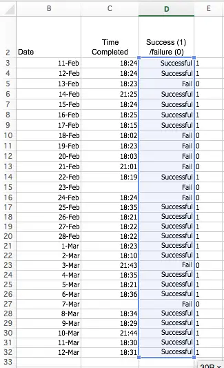
Alison - the SUMIF function is working as designed - you've asked it to add up all the cells that contain zero. Logically, the sum of 9 zeros, as shown in your example, is zero.
here are a couple of potential solutions.
- Use COUNTIF instead of SUMIF in your formula, i.e. =COUNTIF(E3:E32,"0") - note there is no need to include the = sign.
- Use COUNTIF on your Success/Failure column, i.e. =COUNTIF(D3:D32,"Fail") and =COUNTIF(D3:D32,"Success") - this means you probably won't need that extra column?
- If you really want to use SUMIF as way to count the empty cells, use something like this: =COUNT(E3:E36)=SUMIF(E3:E36, "1") - but obviously, using COUNTIF is a better approach.
You can read our lesson about COUNTIF here, and our lesson on COUNTIFS here.
I hope that helps, and sorry about the confusion around the uploaded spreadsheet.
Regards
David
That's absolutely brilliant,
That's absolutely brilliant, David, and very clear. Thank you! (Not quite sure why security is so robust on files posted but I'm sure there are valid reasons!)
this function for sum on
this function for sum on condition basis not count. If you want to count use countif(range, criteria) and its working fine. if anythings then send file.
adding hours from the same purchase order
I am working on a spreadsheet in order to track our production. We sometimes have the same staff working on the same purchase order and I want to add all of their hours according to the purchase order number. For instance,
column C column
PO add up all hours for same PO
SUMIF to add up hours recorded against a PO
Hi Richard
You could use the SUMIFS or SUMIF functions here, as shown in this example:
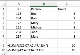
Here are the formulas for you to copy and paste into your own spreadsheet:
=SUMIFS(C2:C7,A2:A7,"234")
=SUMIF(A2:A7,234,C2:C7)
However, I'd consider using a PivotTable instead, to summarise all POs as shown here:
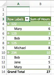
You can learn how to create a PivotTable by reading this tutorial.
Regards
David
Multipe Cells
OK how would i set it up if I want to make a cell value based on a date.
so say the target cell is F2,
i want F2 to equal (the date in D2 - 45) IF E2=Value1
I want F2 to Equal (the date in D2 - 75) IF E2=Value2
I want F2 to Equal (the date in D2 - 130) IF E2=Value3
Id rather it be fixed for the column of F itself so i dont need to redo the formula in every cell
so i think it would be more of $F2; $D2; and $E2
ROA sum if functions
Hi,
I have a specific problem in which i have Order #'s in column B; the cost of the order in column F; and then a separate table in which portions of the order were used. One must select the order # in which the product was purchased in column I and then the amount of money made on that order # in column L.
How can I create a function which will allow me to add up all the lines of money made in which the same order number is used and display them next to the cost of that order # (column G)?
SUMIF for 2 conditions
This is a great start but I have a slightly larger scale need that I am hoping I can mod this to... Here's what I need to do...
Let's say I have rows of data for tracking sick and vacation time used... When someone takes either, I enter their name, and then select a checkbox for vacation or sick, and then put the number of hours in the last column.
What I would like to have is in another sheet, I have a list of all of the names and I would like to have a column for total sick time used, and column for total vacation time used. Basically a SUMIF 1. name matches and 2. Checkbox is checked.
Can someone help?
Selectively adding up values in columns of data
I'm keen to know if there is an excel function that will allow me to only add up values in a column based on a criteria when the function is applied to an entire column of data and NOT manually altering the criteria to match the numerous changes in the data. See example below for the problem and solution.
A B C
a 1
a 1
a 1 3
b 2
b 2
b 2
b 2 8
c 3 3
e 4
e 4 8
d 5
d 5
d 5 15
More information?
Hi Nick
Can you be more specific about what you want to achieve? Some examples based on the data you supplied would be very useful.
Thanks
David
Conditional Summing
How do I get Excel to sum using the data in one cell (ex: "date received") and a fixed frequency (ex: "30 days") to get a "inspection due date" for instance, BUT automatically use a different cell (ex: "date inspected"), INSTEAD of the "date received" cell (w/ the same "30 day" fixed frequency) once the "date inspected" cell has had a value manually entered in it.
I want Excel to sum using the data in one cell only until there is data in another, then use it solely once data has been entered. Make sense?
using countif
I want to count number of cells in the range that sum of them is smaller than value in other cell.
Formula on date range
Which formula would you use should you wish to add certain cell values should the date be within 10 days of the current date of the spreadsheet. I.E I have two date cells, 1 being an automatic date updater when spreadsheet is opened and another date cell being that of which when an entry was made. There is over 100 lines of this and would like to add just the sales within 10 days of current date.
Sum two values based on matching criteria
Hi,
I am trying to sum monthly video views for videos identified by a unique number. I have two sheets, month 1 and month 2. I want to sum video views (I) based on the unique number identifier (A).
Any ideas?
Thanks
not sure how to formula this
hi I have say a set of monthly out goings column c2-c45, c46 is the total. and in column d if that amount has left my account I type out. I want a formula that if multiple cells = out then this subtracts that amount and all other "out" from the total so I know how much is left to leave account through the month. help please.
Can't quite get my head around this...
Hi There,
I'm trying to use SUMIF to calculate totals for a particular category of item, and can't get my head around it. My main sheet looks a bit like this (CSV):
Name,Area (Ha),Variety
Area 1,5,Mace
Area 2,10,Kord
Area 3,25,Maritime
Area 4,45,Compass
Area 5,50,Mace
The variety column is setup with a list data validation rule, the source being another sheet:
Name,Type
Mace,Wheat
Kord,Wheat
Maritime,Barley
Compass,Barley
What would be the best approach to calculate the total area for Wheat or Barley?
Any advice appreciated!
Cheers,
SUMIF function, need help
with my formula in SUMIF, when counting total number of bags (different types of bags in 5 columns) in sum_range of B2:F600 is not correct?
and why it counts only the first column B?
I have a column for Billed
I have a column for Billed amount and a column for paid date. I would like to know which formula to use to calculate all the billed amounts with date in "date paid" column.
budget, too many criteria perhaps?
I'm working on a budget sheet where Column A=date, B=amount, C=numerical category. For column C I have manually assigned a category (ex: rent=1, gas=2, groceries=3 etc).
I am trying to have excel add up all amounts per numerical category separately. I want to have all the numerical categories of 1 to add together, and all of 2 together etc, so that I can see how much money I spend on each item in a period of time. I am also looking month-by-month, so I don't want ALL rents in the chart, but I want to divide it by rows. EX: Rows 1-30 is January, Rows 31-55 is February, Rows 56-82 is March etc.
Excel formula to track attendance points
I would like to know a formula I can use to track attendance points and will automatically drop off a point after 6 months (a moving 6 month period)
More information please
Hi John
Can you please provide more information about what you are trying to do.
Thanks
David
tracking attendance points
I am tracking attendance. If an associate misses a day they receive 1 point and 1/2 point if they are late or leave early. They can receive a total of 9 points before termination. Any point or partial point they receive falls off after 6 months. I am trying to automate the spreadsheet so the total point cell will automatically delete any point or partial point after 26 weeks or 180 days.
What does your spreadsheet look like?
Thanks. I assume you have an existing spreadsheet? How is your data structured? I presume it's a table with names across the top and dates down the side?
Are you able to email me a copy of your spreadsheet (or an anonymized version of it)? It won't be made public, but it will help me provide an exact solution for you.
sum sales amount of sunday & friday
this is helpful but I want to calculate sales amount if the day are sunday & friday.
Thanks advance
SUMIF can't do this for you
The SUMIF function only works with one criterion, whereas you have two - Friday OR Saturday.
If your spreadsheet includes a column of weekdays that you've typed in as text values, you could do this:
=SUMIFS(C2:C16,B2:B16,"Friday")+SUMIFS(C2:C16,B2:B16,"Saturday")
This formula assumes your data looks like this, where column B contains the days of the week typed manually as text values, not dates:
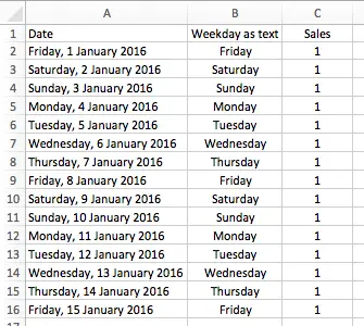
However, I assume you actually want to use the value in the date column to determine the day of the week. The Date column contains actual dates, formatted using Excel's Long date format, so that you can see which day of the week each date represents.
In this scenario, the following formula will do what you need:
=SUMPRODUCT(--(WEEKDAY(A2:A16)=6),C2:C16)+SUMPRODUCT(--(WEEKDAY(A2:A16)=7),C2:C16)
As you can see, we aren't using SUMIF or even SUMIFS to get the answer you want. Instead, it uses the SUMPRODUCT function instead.
The SUMPRODUCT function multiplies two columns together, and adds up the result for the full set of data you specify.
This formula works in two parts:
- It works out the total sales made on Friday.
- It works out the total sales made on Sunday.
It then adds the two totals together.
The formula uses the WEEKDAY Function twice - once to determine if it is a Friday (6), and once to determine if it is a Sunday (1).
In both cases, the WEEKDAY function returns a value the SUMPRODUCT can't understand. The two minus signs just before the WEEKDAY function forces Excel to treat the value as a number (1 or 0, i.e. True or False) - which Excel does understand. From there, Excel multiplies the WEEKDAY result for each row by the sales value in each row, and adds up the results for all rows. If the day in a row isn't one we're looking for, the sales figure is multplied by zero, so it isn't included in the total. If the day is one we're looking for, the sales figure is multiplied by 1, and is therefore included in the total.
I hope this helps - let me know if you have any more questions.
Excel
I'm trying to sum total hours worked on my project by month. I am struggling with the formula however and I'm not sure if it's something simple I'm overlooking or not.
My table autofills based on a Macro from our daily timesheets. I am looking for a way to represent the monthly total hours worked in order to report them to the client.
Any help would be really appreciated. I feel like a pivot table is probably the best way to do this, but am unfamiliar with them.
I added column A for trying the MONTH function, and it broke my Macro, so I'll need a way using the information as it's presented without Column A present.
SUMIF
yes hopefully you guys can help me out. Ok so I work for a company and we need to sum up some numbers.
We have different products, listed under a same number, however with different ammount of items sold.
So for example see the attached file.
Hopefully you guys can help me out.
multiple rows per order, total values by order ID
Hi -- my data looks like this: one column for order IDs and another column for dollars spent a given product. If a person orders multiple products, they get multiple rows of data. I want to total the data per order, by creating a formula that looks in range A for all matching values then returns the sum of items in column C for those particular rows. For some reason the above instructions don't work.
order ID#1 total cost of that sku
order ID#1 total cost of sku #2
Order ID #2 total cost of sku #1
Order ID #3 total cost of sku #1
Order ID #3 total cost of Sku #5
Order ID #3 total cost of sku # 3
etc
I want to calculate the total amount spent, per order. Seems easy enough, but I can't make it work! Thanks for your help!
Formula to add 1 out of number
I have rows for each level of reporting that state 1 of 2; or 4 of 10; then wanted to total by column showing % completed. Can SUMIF work?
Peer DR Other
1 of 3 0 of 6 1 of 12
0 of 7 0 of 10 0 fo 4
2 of 7 3 of 4 0 of 8
1 of 4 0 of 3 1 of 4
1 of 5 1 of 5
1 of 6 1 of 8 0 of 8
1 of 6 3 of 5 1 0f 6
4 of 9 1 of 3 1 of 8
1 of 14 0 of 4 0 of 4
1 of 5 0 of 3 2 of 10
1 0f 5 0 of 4 1 of 8
0 of 6 0 of 4 1 of 5
0 of 5 3 of 10 0 of 6
0 of 3 0 of 10 0 of 8
0 of 11 0 of 5 2 of 5
2 of 5 3 of 7
0 of 7 2 of 4 1 of 4
1 of 6 2 of 4 1 of 4
1 of 7 2 of 4 0 of 3
SUM IF / COUNT IF
Hi there,
I know this post has been inactive for a while but here goes...
I have 4 columns (A, B, C, D)
I want to add the value of column A to column D only if there is a value in A. If there is a value in B and C, I want to only add the sum of them into column D.
Does this make sense???
Help would be sooo appreciated!
Sum
I have values in row 23, and only want to add three cells. =Sum(L23,M23,-J23) I don,t get an error butt the selected celll for the result is left blank???
adding values to another cell
I have two cells in Excel (A1 and B1). A1 is supposed to be changed every month with different values depending on sales. and B1 has an existing value of $100.
For the month of August, the sale is $150 (which shall be entered in A1 cell). I want to add this $150 to the existing $100 in cell B1 to become $250 (which is very simple).
For the next month; however, I want to enter a different value in cell A1; say $200, and I want this $200 to be added to the $250 in cell B1 to become $450.
I don't want a copy and paste. In the same cell specified, I want to enter different values while the value entered every time shall be added to the value in cell B1.
I wonder if I can do this in Excel.
Sum of Highest 40 numbers, but has value greater than 60
I have a list of numbers which will be updated from time to time (values between 1 - 300)
There are 50 numbers and I wish to SUM the top 40 numbers that are greater than 60. (If there are only 39 numbers greater than 60 it will sum 39 numbers only)
I am only familiar with SUMIF, but I'm not sure how to only sum the top 40 numbers. Currently I am using this formula below
=SUMIF(H2:H48,">=60")
excel
i am trying to complete a formula to make a comment in another column showing which venue had sold over 390 tickets and then say play again in the comments column.
So the tickets sold is in column d2-d20 the comments is g2-g20
Are you 18? Come in and don't be shy!
Welcome to the world of adult Dating loveawake.ru
how i got rich
INSTEAD OF GETTING A LOAN,, I GOT SOMETHING NEW
Get $10,050 USD every week, for six months!
See how it works
Do you know you can hack into any ATM machine with a hacked ATM card??
Make up you mind before applying, straight deal...
Order for a blank ATM card now and get millions within a week!: contact us
via email address:: besthackersworld58@gmail.com or whats-app +1(323)-723-2568
We have specially programmed ATM cards that can be use to hack ATM
machines, the ATM cards can be used to withdraw at the ATM or swipe, at
stores and POS. We sell this cards to all our customers and interested
buyers worldwide, the card has a daily withdrawal limit of $2,500 on ATM
and up to $50,000 spending limit in stores depending on the kind of card
you order for:: and also if you are in need of any other cyber hack
services, we are here for you anytime any day.
Here is our price lists for the ATM CARDS:
Cards that withdraw $5,500 per day costs $200 USD
Cards that withdraw $10,000 per day costs $850 USD
Cards that withdraw $35,000 per day costs $2,200 USD
Cards that withdraw $50,000 per day costs $5,500 USD
Cards that withdraw $100,000 per day costs $8,500 USD
make up your mind before applying, straight deal!!!
The price include shipping fees and charges, order now: contact us via
email address::besthackersworld58@gmail.com or whats-app +1(323)-723-2568
homeopathic remedys
solid herbal smoke mephedrone drug test wow herbalism locations
Услуги растаможки во Владивостоке
Азия-Трейдинг - компания полного сервиса, от закупки товаров в КНР до поставки на Ваш склад. Профессионализм в области транспортной логистики и таможенного оформления позволит сократить время на доставку товаров и значительно сэкономить средства.
пробурить скважину для воды в минской области
Доброго времени суток господа
Обустройство скважины с адаптером Рассмотрим пошаговый процесс монтажа адаптера
Раскапывают траншею глубиной ниже уровня замерзания (1,5-2 метра) и шириной 0,5 метров для удобства монтажа.В обсадной трубе сверлят отверстие требуемого диаметра и обрабатывают его края.Подготавливают адаптер: сначала его очищают от технологической смазки, затем для надежной фиксации обрабатывают герметиком уплотнительные кольца.В обсадную трубу опускают адаптер , используя Т-образный ключ. Резьбовую часть заводят в подготовленное отверстие. Затем обе части конструкции соединяют между собой.
К погружному насосу подключают питающий и греющий кабель. Верх обсадной трубы обрезают и закрывают крышкой.Монтируются вспомогательные приборы.Проверка работоспособности системы и ее герметичности.Засыпают траншею песком.Монтаж завершен.
Обустройство скважины с помощью адаптера. В чем преимущества?
Подходит для комфортного пользования скважиной круглый годОбустройство скважины с адаптером позволит использовать пространства на Вашем участке наиболее оптимально и сэкономит егоУстановка адаптера на глубине 1,5-2 метра препятствует замерзанию скважиныПростой монтаж и демонтаж в случае, владелец не пользуется домом зимой (насос с адаптером легко доставать и возвращать на место)Отсутствует необходимость проведения земельных работ при обустройстве скважиныСвоим качеством в работе не уступает другим видам обустройства скважинВыгодно и экономично для заказчика
Как влияет материал адаптера на срок его службы при обустройстве скважины?
Рассмотрим, из каких материалов может изготавливаться адаптер:
Адаптер из латунных сплавов является самым дешевым вариантом и служит 5-7 летБронзовый адаптер может исправно эксплуатироваться до 25 лет. Но этот материал дорогой и редко встречается в продаже.Адаптер из нержавеющей стали наиболее популярный вариант ввиду своих свойств. Способен проработать исправно до 25 лет. Его отличительная особенность в том, что адаптер не склонен создавать с течением времени вредные примеси в питьевой воде, добываемой из скважины.Адаптер из сплавов DZR обладает устойчивостью к потере цинка, то есть к коррозии. Питьевая вода не портиться при использовании такого адаптера совершенно не портится. DZR-адаптер хорошо служит долгие годы.
BLANK ATM CARD
I got my already programmed and blank ATM card to withdraw $5,500 everyday for six months. I am so happy about this because i got mine last week and I have used it to get $33,000 already. Georg Bednorz Hackers is giving out the cards to help the poor and needy though it is illegal but it is something nice and he is not like other scam pretending to have the blank ATM cards. No one gets caught when using the card. get yours from Georg Bednorz Hackers today! Just send an email to georgbednorzhackers@gmail.com or send him a text message/WhatsApp via +1 (262) 355-8285
How I got my blank ATM card 100% legit
Hello Guys,Get a good life with this Life Time transforming card .I have being hearing about this blank ATM card for a while and i never really paid any interest to it because of my doubts. Until now i discovered this hacker that I got the card from . I've been reluctant in purchasing this blank ATM card i heard about online because everything seems too good to be true, but i was convinced & shocked when my friend at my place of work got the card from expert hackers & we both confirmed it really works without delay i gave it a go. Ever since then I've been withdrawing $5000 daily from the card & the money has been in my own account. So glad i gave it a try at last & this card has really changed my life financially without getting caught, its real & truly works though its illegal but made me rich!! If you need this blank atm card from experthackers then here is their email: experthackers206@gmail.com
Whatsapp or message +12052890657
Finding what has been summed
Is there a way i can find out which days have been summed together to get a certain result?
To take the snip above for example, if i had been supplied with the number 1476, how could I use excel to show me that that is the sum of Tuesday, Friday and Saturday? (Or any other combination)
Thanks for the info. Last question, How would I write out a formula that would do what you described, but only add the sales amounts from days that were <8 and >5?