Use INDEX to lookup multiple values in a list
Excel's VLOOKUP function is excellent when you want to find a value in a table based on a lookup value. But if your table includes your lookup value multiple times, you'll find that VLOOKUP can't do it. This lesson shows you how to use the INDEX function (plus some other functions) to find all matching values in a list, and return a value from another column in the same row. It also looks at how to do this when you want to return all values which are a partial match (i.e. a wildcard search) to the values in your lookup table.
Here's a simple example based on a question I was asked by one of our readers.
- There are two worksheets, one containing Form data for a mail merge, and one containing Parcel data, some of which is to be included in the mail merge.
- The Form worksheet includes a row for each landowner who is to receive a letter. One of the columns in the spreadsheet is an ID for each landowner.
- The Parcel worksheet contains data about land parcels owned by the landowners in the Form worksheet.
- The mail merge will generate a letter to all land owners. That letter should include details of all of the land parcels owned by that individual land owner.
In this lesson I'm going to focus on how to include that land parcel information in the mail merge, but I'm not going to discuss how to set up the mail merge with Microsoft Word.
Use the Index function to return multiple values a list
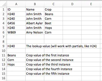
Let's say our Parcel worksheet looks like this:
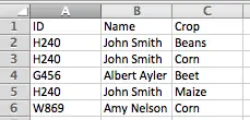
As you can see, John Smith (ID H240) appears three times. We want to include a list of the crops John grows in our mail merge letter. If you've used a VLOOKUP function before, you'll know that we can use it to find the first crop for John in the list, but not the second or third.
Find all the row numbers to match our lookup value
Let's start solving our problem by first finding the row number of each row in which H240 appears, by using the formula below. After that we'll then extend this formula to find the crop value in each row:
{=SMALL(IF($A$2:$A$6=$A$9,ROW($A$2:$A$6)),ROW(1:1))}
Here is a breakdown of this formula:
- The { } around the formula indicates that this is an array formula.
- Note that you don't type these braces as part of the formula. You have to press Ctrl+Shift+Enter key when entering the formula to tell Excel it is an array formula, after which the { } will automatically appear. If you don't, our formula will return a #VALUE error.
- If you're using Excel for Mac, you'll need to press CMD+SHIFT+Enter instead.
- The SMALL function has the syntax SMALL(array,k).
- It looks up a list and finds the k'th smallest value in the array.
- If k = 1 it will find the smallest. If k=2 it will find the second smallest value, and so on.
- The second instance of the ROW function is used to find k in our formula. In this example, ROW will return the row number of row 1, which is, of course, 1.
- The IF function looks to see if the value in A9 is in the list.
- In our example, A9 is where we'll enter H240 as our lookup value.
- Note that the IF function will only return a value if our number is in the list.
- If not, it will return a null value, which will cause the SMALL function to generate an error. We'll look at how to hide that error later.
- The ROW function is used twice:
- If the IF function finds our value in the list, the ROW function returns the row number in which it was found. Note that it returns the row number of the worksheet, not the row number inside our table. This will be important later.
- As noted above, the ROW function is also used in our formula to return k.
The screenshot below shows this formula in action:
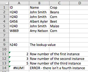
In the screenshot above, I've entered h240 into A9 (you'll note that our formula isn't case sensitive). I've then entered the formula above into A11 as an array formula (don't forget that part!). It has returned 2, which is the row number for the first instance of H240 in the list. After that, I've copied and pasted the formula into rows A12 to A13. The formula has automatically picked up the correct row numbers, and generated an error when it couldn't find a fourth value.
However, there has been some magic under the hood that you can't see here. When I copied and pasted the formula into the additional rows, the array formula changed. Here are the formulas in each cell:
{=SMALL(IF($A$2:$A$6=$A$9,ROW($A$2:$A$6)),ROW(1:1))}
{=SMALL(IF($A$2:$A$6=$A$9,ROW($A$2:$A$6)),ROW(2:2))}
{=SMALL(IF($A$2:$A$6=$A$9,ROW($A$2:$A$6)),ROW(3:3))}
{=SMALL(IF($A$2:$A$6=$A$9,ROW($A$2:$A$6)),ROW(4:4))}
Note how the ROW parameters in each formula are different: 1:1, 2:2, 3:3, 4:4. This is telling the SMALL function to find the 1st, 2nd, 3rd and 4th values in the list that match our lookup value. As I said, you don't need to edit the formula yourself - it updates itself when you copy and paste it.
Use the INDEX function to find the Crop values
Now that we know the row numbers for each instance of H240 in our example, we can use the INDEX function to use the row number in order to obtain the Crop value. If you're not familiar with the INDEX function, you can read our lesson on INDEX here (it will open in a new tab).
Here's the adjusted formula:
{=INDEX($A$2:$C$7,SMALL(IF($A$2:$A$7=$A$9,ROW($A$2:$A$7)),ROW(1:1))-1,3)}
Here's how this function breaks down:
- The INDEX function looks in our table ($A$2:$B$7)
- It then uses the SMALL function to find which row to look in and then subtracts 1 from what SMALL tells us.
- Remember that the ROW function returns the row in the worksheet where our value was found.
- The INDEX function considers the first row of our table as row 1. Because our table data starts in row 2, we need to subtract 1 from the ROW value to get the correct row inside the table.
- If you're applying this solution to your own spreadsheet, you may need to adjust this value to take account of where your data table is located.
- The INDEX function then looks in column 3, which is where the crop data is found.
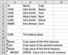
Here's how our spreadsheet looks now.
Hide errors generated by our formula
At this point, we've done what we set out to do, which was find all of the crops related to John Smith. However, if we are going to use this solution in a mail merge, we don't want the mail merge to print #NUM in our letters. Let's finish off this lesson by looking at how you can hide error values when they occur in our formula:
{=IF(ISERROR(INDEX($A$2:$C$7,SMALL(IF($A$2:$A$7=$A$9,ROW($A$2:$A$7)),ROW(1:1))-1,3)),"",INDEX($A$2:$C$7,SMALL(IF($A$2:$A$7=$A$9,ROW($A$2:$A$7)),ROW(1:1))-1,3))}
This formula looks terrifying, but it's actually very simple.
- The IF function tests to see if our formula generates an error. It does this by using the ISERROR function.
- If the ISERROR function is true (i.e. our formula generates an error) then the IF function returns "", which means the cell containing our formula will appear to be blank.
- If the ISRROR function is not true, then our formula works OK, and the IF function will use it to return the correct value.
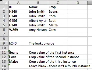
There's not much to see when we use this version of the formula, but here is what our spreadsheet looks like now:
Finding all matching values using partial match
A couple of people have asked in the comments below whether there was a way to use a wildcard, or partial match, for the lookup value in A9. The answer is yes - and here's the formula to use - you can replace the array formula in A11:A14 in the example above:
=IF(ISERROR(SMALL(IF(IF(ISERROR(SEARCH($A$9,$A$1:$A$7)),FALSE,TRUE),ROW($A$1:$A$7)),ROW($C$1:$C$7))),"",INDEX($A$1:$C$7,SMALL(IF(IF(ISERROR(SEARCH($A$9,$A$1:$A$7)),FALSE,TRUE),ROW($A$1:$A$7)),ROW($C$1:$C$7)),3))
This formula uses the SEARCH function to determine if the lookup value in row 9 can be found in the cells in A10. In practical terms, this formula allows you to type a partial match, e.g. H24, and the formula will return all instances where H24 is found in column A. Note that you don't need to use asterisks, *, to indicate to Excel that you are using a wildcard - you simply type the partial string you want to match.
Note that there is a twist in this final example. You can't copy and paste the formula from A11 into A12 - A14 as you could in earlier examples. You have to do the following:
- Get the array formula working in A11, and returning the correct result (Beans in my example).
- Select all the cells where you want this formula to be (including the cell with the first working example). In my example it is A11:A14. Make sure the active cell is the one containing the formula.
- Click in the formula bar to start editing the formula but don't change anything.
- Press the keys to enter an array formula (CTRL+Shift+ENTER on PC or Command+Shift+Enter on Mac).
- The selected cells will change to show you the correct results, and the selected cells will become an array.
Once you do this, the selected cells can only be treated together as an array. If you try to edit, say, A13, you'll get an alert telling you that you can't edit an array. If you want to change your formula, you need to select all of the cells in the array, click in the formula bar, and then press the keys to re-enter the formula as an array formula. If you simply want to break the array, select all of the cells, click in the formula bar and press Enter.
Summary
And with that, we're finished. If you have any questions about this solution, please let us know in the comments!
* This lesson was inspired by a post by Ashish Mathur for Excel 2003. You can read that post here. The inspiration for this lesson came from a question from one of our readers on the original lesson on how to use the INDEX function. The formula for using a wildcard came from this forum discussion. All links open in a new tab.
Download worked examples
Join our mailing list
Our Comment Policy.
We welcome your comments and questions about this lesson. We don't welcome spam. Our readers get a lot of value out of the comments and answers on our lessons and spam hurts that experience. Our spam filter is pretty good at stopping bots from posting spam, and our admins are quick to delete spam that does get through. We know that bots don't read messages like this, but there are people out there who manually post spam. I repeat - we delete all spam, and if we see repeated posts from a given IP address, we'll block the IP address. So don't waste your time, or ours. One other point to note - if you post a link in your comment, it will automatically be deleted.
Comments on this lesson
VLOOKUP should work for this scenario
Hi Michael
I recreated your spreadsheet and verified that VLOOKUP will work in the scenario you've described. I don't see anything in that would require you use the INDEX function in the way it's used in this lesson.
The only potential problem I can see is if you want someone to type a year, e.g. 2020, rather than the range shown in your table above, either 2019/20 or 2020/21. In that case, this scenario won't work because VLOOKUP is looking for a match between what is typed in C14 and the values in the first column of your table. A value like 2020/21 is treated as a text value by Excel, so the text you type into C14 must match that text value.
If you want someone to be able to type 2012 and have the formula return the correct result, you'll need to respecify the data table so the first column matches the potential values the users might type, i.e. 2013, 2014, 2015 etc.
If you're unable/unwilling to respecify the values in the table, you could respecify the lookup value. The following formula shows a calculation that will take a year, e.g. 2013, and convert it into a text value (2013/14) so that it can be used in your VLOOKUP function.
=C12&"/"&C12-1999
What it does is take the value in C12 and creates a text value by concatenating additional characters, starting with a / symbol, followed by another number. That number is the value in C12 (e.g. 2013) less 1999 (which gives us 14). So the result would be 2013/14, which is a text value. If you use this as the lookup value in VLOOKUP, it should return the result you want.
I hope this helps!
Regards
David
Great Infomation !
Thank you for giving me the opportunity to visit this impressive website. There is plenty of valuable info listed on this site.
I have seen a lot of tricks. It is too much to absorb at once, thus I definitely will return to view more
http://www.jumbojobs.com/seo-jobs
Expanding the INDEX function
Hi,
Thank you ever so much for the above - very helpful!
I was just wondering if you might be able to help me expand the formula somewhat? I am interested in combining this with another IF and checking against an additional column e.g. if column A = M AND column B = Y then use INDEX to find the different values e.g. the first instance of Y=Z, the second instance of Y=Z, the first instance of Y=T, the second instance of Y=T, the third instance of Y=T etc…
For reference, within this worksheet: Column A contains my references (the Ms mentioned above) and row 3 contains the numbers 1, 2, 3 etc. for the ROW(1:1) part e.g. first, second, third instance (I am dragging my formula horizontally rather than vertically as in your example above). Row 2 contains the Y criteria.
In the other worksheet (containing the data I want to search through): Column_A is the column containing the Column A values from the previous sheet (the Ms) and Column_B contains the second search criteria. Search_Area is the full table. Header_Row is the header row and “X” and “Y” are some of the column labels.
My original formula is:
=IF(ISERROR(INDEX(Search_Area,SMALL(IF(ISNUMBER(SEARCH($A6, Column_A)),ROW(Column_A)),ROW(INDIRECT(B$3&":"&B$3))),MATCH("X", Header_Row,0))),"",INDEX(Search_Area,SMALL(IF(ISNUMBER(SEARCH($A6,Column_A)),ROW(Column_A)),ROW(INDIRECT(B$3&":"&B$3))),MATCH("X",Header_Row,0)))
I’ve expanded it to:
=IF(ISERROR(INDEX(Search_Area,SMALL(IF(ISNUMBER(SEARCH($A6,Column_A)),ROW(Column_A)),ROW(INDIRECT(P$3&":"&P$3))),MATCH("X",Header_Row,0))),"",IF(INDEX(Search_Area,SMALL(IF(ISNUMBER(SEARCH($A6,Column_A)),ROW(Column_A)),ROW(INDIRECT(P$3&":"&P$3))),MATCH("Y",Header_Row,0))=P$2,INDEX(Search_Area,SMALL(IF(ISNUMBER(SEARCH($A6,Column_A)),ROW(Column_A)),ROW(INDIRECT(P$3&":"&P$3))),MATCH("X",Header_Row,0)),""))
But it only works if the first value is Y=P2 which it isn’t always! Is there a way to achieve this without splitting out all of the data into separate worksheets?
Many thanks!
can i use this lesson with a "Column" instead of "ROW"?
hello
i have the following row that includes 9 names (per working day). i can't know the names in advance, and there might be the same guy appearing twice.
below that row i have another one with the kilometers each guy drove.
for example:
Nick | Henk | Sidney | Nick | Roberth | Mark (so as you can see Nick is there twice, becasue he worked 2 days in that week).
100 | 210 | 150 | 190 | 45 | 76
i total, i will have 52 rows with names and 52 rows with KM, to cover the whole year...
i want to have a side table to show me how mny KM each guy did on every week.
so in the above example i'd like to have this:
week 1 - Nick | Henk | Sidney | Nick | Roberth | Mark
KM - 290 | 210 | 150 | 190 | 45 | 76
so as you can see, Nick's result was 290 (100+190) becasue he worked twice.
i thought your trick with the INDEX and ROW was almost what i need, but i think i have to find the occurences of "NICK" looking DOWN, right?..
please help!... :(
thanks!
Ran
A simple SUMIF function should do what you need
Hi Ran
It looks like you can do what you need with a simple SUMIF. People tend to think of SUMIF as being used for adding up data in columns, but it works just as well to add up data in rows provided you set it up correctly.
Let's work with this example from the spreadsheet you provided.
Here's the source data:
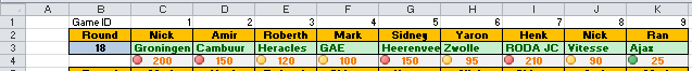
Here's where you want to calculate the results. The table starts in M13 with Amir's name (it's a little confusing, but the 18 in this picture refers to the Round from the picture above, not the row number in Excel):
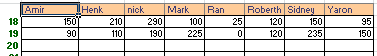
The formula in round 18 for Amir is this:
=SUMIF($C2:$K2,M$13,$C4:$K4)
This formula looks in the cells from C2:K2 (the names in the table) and matches them with the value in M13 (Amir). If there is a match, it adds in the calue from the appropriate cell in the range C4:K4 (kilometers driven by that person).
I've written this formula using a mixture of absolute and relative references so that you can copy and paste it from Amir to Yaron without changing it. However, the layout of your spreadsheet means that you can't just copy the same formula down to Round 19 without adjustment.
Here's how the formula in Round 19 would need to look:
=SUMIF($C5:$K5,M$13,$C7:$K7)
As you can see, I've had to adjust the range references (e.g. $C2:$K2 became $C5:$K5), but not the reference to Amir's name (M$13).
I hope this helps. Let me know if you still have any questions.
You can read more about the SUMIFS function in this lesson.
Regards
David
THANK YOU!
indeed, you are right! i guess i was complicating things unnecessarily...
talking about this same spreadsheet, i have another question if you don't mind, in related to using of "IF"...
in the attached file, i added another list. i want to see which operator worked at the following stadiums (Groningen, Roda JC, Cambuur).
so i used this formula to search within the data of round 18:
=IFERROR(INDEX(C2:K2,MATCH($N$2,C3:K3,0)),"")
so N2 = Groningen in that case.
now, if i want to auto copy this to all the way to the bottom, to cover rounds 19,20,21, etc etc, i can't use the drag method (from the corner of the cell), because it will increment the C2:K2 to be C3:K3. while i actually need it to be C5:K5... (this is where the data of round 19 is).
so me question is:
1- how can i tell Excel to auto-increment by 3 numbers? so to jump from C2 to C5 to C8 etc etc?
2- if the above question is not possible,how can i add another "MATCH" parameter to also check the round number?
for example:
Match N2 (Groningen), but also match the round number (for example M6, M7 etc etc)?...
i hope i explained my self correctly...
many thanks for helping so far!
Ran
HELP!
Basically, I'm creating a group registration form wherein each person can register for multiple events (77 choices). I will be leaving several columns for them to fill the events they want to register for. So each form will have multiple names, each name having several items attached to it.
Post-registration, I would need to be able to pull out the list of people who registered for each event. Can I alter this formula to work for me? The main issue is people can register for the same events but end up typing it in the a different column since I'm leaving several open. If so, how? I attached a sample sheet. Appreciate any help I could get on this matter.
Almost there!
Hello! I have your website to be of the utmost help. I appreciate the time you put into it, so thank you for that. I am writing as I'm pulling my hair out trying to figure out my work.
I have two tables, one on sheet1 and the other on sheet2. They are setup in identical position, and their headers are identical. What I am looking to do is:
1. find where in the first table a variable occurs (say variable a1).
2. Count the instances of each unique variable. (I've accomplished this with copy and paste from pivot tables)
3. if variable a1 occurs three different instances in the first table, I would like to extract the corresponding data from table 2, that is in the exact same row/column as variable a1 - table2 holds an index of sorts.
here would be an example (aside from the file I uploaded):
table 1
header1 header2 header3
row1 a1 a2 a3
row2 a2 b1 a1
table2
header1 header2 header3
row1 1 2 3
row2 4 5 6
My goal is to output this:
variable occurance index1 index2
a1 2 1 6
a2 1 2...
any input would be greatly appreciated! I tried to capture the row and column of each variable, however the COLUMN function isn't behaving the same as the ROW function. I keep getting returned the COLUMN for the first occurance of the variable.
What happens if the value of the cell contains a blank?
Hi - this lesson really helped me and I was able to modify it for what I need, but I have one question - if one of the cells that the formula picks up, is blank but I still want it to show on my new worksheet as a blank in that cell, how do I write this into the formula?
Taking your example - looking at row 5 - A5 ID is H240, B5 is John Smith but C5 was blank, how do I get it to show as a blank cell - it currently returns a "0" or if formatted as a date field "00/01/1900". If you can help - this formula would be perfect for what I need! Many many thanks!
Add an extra IF function to test for zero
Hi Nikki
What you need is actually pretty simple - simply add another IF function in to check if the result is 0, and output a blank cell if it is. Here's the formula to use in the example above:
{=IF(ISERROR(INDEX($A$2:$C$7,SMALL(IF($A$2:$A$7=$A$9,ROW($A$2:$A$7)),ROW(1:1))-1,3)),"",IF(INDEX($A$2:$C$7,SMALL(IF($A$2:$A$7=$A$9,ROW($A$2:$A$7)),ROW(1:1))-1,3)=0,"",INDEX($A$2:$C$7,SMALL(IF($A$2:$A$7=$A$9,ROW($A$2:$A$7)),ROW(1:1))-1,3)))}
All I've done is put another IF function into the formula (highlighed in bold). So the formula does this:
- Check if the INDEX function returns an error. If so, return "" (a blank cell)
- If it doesn't return an error, check if the INDEX function returns a zero. If so, return "" (a blank cell)
- If it doesn't return a zero, return the value from the INDEX function.
I hope that gives you what you need!
Regards
David
(p.s. I also fixed an error in the final part of the original lesson where I added error checking)
skip instead of blanking
Hi, David, Is there a way to make it skip this blank cells or the zero values themselves? this works almost as I need it to work, the only problem is, I just want the data, I made an offset chart with paired with this formula, the problem is, the chart shows all this extra series that cointain purely zeroes, this is no problem, the chart shows the actual info I need, but for instance, you need to hover over the chart lines in order to know exactly the data is showing, and if I could filter this zeroes without using filters of course, that would be great.
returning multiple answers
I've read your comments on using 1 item to bring in multiple corresponding answers, but can this same approach be used for multiple items to bring in multiple answers? On the example attached, the first column is the item name. The 2nd column I've concatenated the quantity arriving with the expected arrival date. Is there a why to use a vlookup on a huge number of items not just one? I have thousands of items repeating with different quantities arriving on different ship dates. thanks.
Mistake in the INDEX formula?
Hello all,
As it seems vlookpu helps me only so far so I started looking for a solution to similiar problem my company has and the solution seems to be the formula mentioned here "Use the INDEX function to find the Crop values" of course adjusted to the values of my company. As I am quite new to the array formulas I started from the scrap a tried to recreate the formula mentioned here:
{=INDEX($A$2:$C$7,SMALL(IF($A$2:$A$7=$A$9,ROW($A$2:$A$7)),ROW(1:1))-1,3)}
for some reason it will not work as the attached example shows. Please be so kind see the file and let me know what I am doing wrong.
It might as well be that this formula does not help my original problem either so here is what I am looking for:
Company name Contract number Employee assigned to work the contract
Company1 Contract001 Employee 1
Company1 Contract002 Employee 1
Company 2 Contract006 Employee 1
Company 3 Contract009 Employee 2
Company 4 Contract 010 Employee 3
What I need to have is that if I put the company name into a cell, that it shows all the contracts this company has opened with us and that it also shows the person that worked this contract in the past and automatically assigns the employee to it or viceversa, if I put the contract number that it always shows the company name related to it and the employee who worked the contract/customer in the past.
Vlookup would work for me only if there always was "one company with one contract" kind of scenario. The problem is that most of the companies have more contracts opened with us and vlookup shows only one contract but is able to assign the right person to it.
I hope this description is enough to understand my demands on the formula and I am convinced that the formula I am trying to recreate in the attached sheet will do once I see where I did the mistake.
Thank you in advance
Regards
Ondrej from the Czech Republic
Mistake in the INDEX formula? attached file
Please see the file
Thank you very much for the
Thank you very much for the article, it worked very well.
I was wondering if there is a modification to pull the list horizontally instead of vertically.
What if I do not want to copy paste formula
What if I do not want to copy paste the formula and just want all the values corresponding to H240 in the column. This is because I might have a column with 1000 rows and I want all the values corresponding to a lookup value in a particular column. Any way this can be done?
Multiple lookup values
Great article! Very clear and easy to follow.
I have a question on whether a variation of this solution is possible to solve my requirement. Your solution works when there is 1 lookup value.
Let's call this lookup value, "ABC123". So, right now I have a worksheet populated with all the data I have configured to be displayed based on the lookup value, "ABC123", present in each row. However, when the lookup value changes (to say, "DEF456") no more data is extracted. I am aware this occurs because of the ROW(1:1) function. Once the lookup value changes the ROW(1:1) function.
Let's look at this with some dummy data so it is clearer. Say I have 5 rows with the lookup value, "ABC123", and another 5 rows with the lookup value, "DEF456". The ROW function will be ROW(5:5) when we come to the fifth row and other indexed data will be displayed in rows 1 to 5. On row 6 the lookup value changes to, "DEF456". The ROW function will be ROW(6:6) and no indexed data will be displayed in rows 6 to 10.
My question is whether there is a formula that will pull all the data and consolidate them regardless what the lookup value might be. Right now, if I want this information I will have to apply the formula separately to the indexed table whenever the lookup value changes.
Any advice you could provide would be much appreciated.
Cheers!
Four years late, but still
I am solving this problem now, I think you could use if function for the row(1:1) problem, so it would look something like this: if(Cell1=Cell2,row(1:1),row($1:$1)). Hope it gives you some joy. Maybe you're still trying to solve it, who knows?
Looking for multyiple occurances of strings withion cells
Hi
I've looked at many web sites looking for an answer to this. I have tried this solution but it is not working. You explain formulas with a good level of detail, thank you, so hence I have a question. I have workbook1 with a sheet (sheet1) containing 6000 rows, 1 column has a product description and a 2nd column has a code number for each description. I also have 6 further work sheets (sheetOTH) that contain a column with a short description. Sheet1 is the client and sheetOTH are suppliers. The descriptions in each sheet are not the same though the descriptions in sheetOTH do appear in part of the description of sheet1. My challenge is to find all the occurrences of the short descriptions from sheetOTH that appear in sheet1 and return the codes from sheet1 to sheetOTH. The aim is to look at each occurrence and match lines in sheet1 with corresponding lines in sheetOTH.
I thank you in anticipation.
1 addition: remove repeated crops
Great example! However, I need to remove repeated occurances of the same return. For instance, if "beans" shows up 5 times, I only want to list it once. So:
Beans
Beans
Beans
Corn
Maize
Beet
Corn
Would return a list of "Beans, Corn, Maize, Beet".
Any idea?
Remove Duplicate Return values
Great example. However, I was wondering if there is a way to remove duplicate items from being returned. For instance, if "beans" occures more than 1 time in the list, can you return the value only one time?
So if the list is:
beans
corn
maize
beans
beans
beets
corn
the list of values returned are "beans", "corn", "maize", "beets" without repeated entries?
PS: apologies if this is a duplicate post, the earlier post seems to have disappeared. (???)
sumif returns 0 though it is not 0
I have a problem in excel.my excel workbook has a sheet (1), which have number in j5. In k5 there long if formula , which calculate data from j5 , =IF(J5<1,"0",IF(J5<11,"2",IF(J5<21,"4",IF(J5<31,"6",IF(J5<41,"8",IF(J5<51,"10",IF(J5<61,"12",IF(J5<71,"14",IF(J5<81,"16",IF(J5<91,"18",IF(J5<101,"20",IF(J5<111,"22",IF(J5<121,"24",IF(J5<131,"26",IF(J5<141,"28",IF(J5<151,"30",IF(J5<161,"32",IF(J5<171,"34",IF(J5<181,"36",IF(J5<191,"38",IF(J5<201,"40",IF(J5<211,"42",IF(J5<221,"44",IF(J5<231,"46",IF(J5<241,"48",IF(J5<251,"50",IF(J5<261,"52",IF(J5<271,"54",IF(J5<281,"56",IF(J5<291,"58",IF(J5<301,"60",IF(J5<311,"62",IF(J5<321,"64",IF(J5<331,"66",IF(J5<341,"68",IF(J5<351,"70",IF(J5<361,"72",IF(J5<371,"74",IF(J5<381,"76",IF(J5<391,"78",IF(J5<401,"80",IF(J5<411,"82",IF(J5<421,"84",IF(J5<431,"86",IF(J5<441,"88",IF(J5<451,"90",IF(J5<461,"92",IF(J5<471,"94",IF(J5<481,"96",IF(J5<491,"98",IF(J5<501,"100",IF(J5<511,"102",IF(J5<521,"104",IF(J5<531,"106",IF(J5<541,"108",IF(J5<551,"110",IF(J5<561,"112",IF(J5<571,"114",IF(J5<581,"116",IF(J5<591,"118",IF(J5<601,"120",IF(J5<611,"122",IF(J5<621,"124",IF(J5<631,"126",IF(J5<641,"128","T"))))))))))))))))))))))))))))))))))))))))))))))))))))))))))))))))).
In another sheet named April in n5 cell i have =IF('(1)'!$A$5:$A$20905=APRIL!$A5,(SUMIF('(1)'!$I$5:$I$20905,APRIL!$M$1,'(1)'!$K$5:$K$20905)),0) formula. This always returns 0, whether k5 has anything. Can you help me?
Better alternatives to Nested IF
Hi DOCKHEM,
There are better alternatives to your nested if in your worksheet. Try below
http://crispexcel.com/6-alternatives-to-nested-if-function/
you can use vlookup instead of so multiple if condi
you can use vlookup instead of so multiple if condition as
VLOOKUP(J5,$O:$P,2,1) where j5 your no and in O:P give range as
O P
0 0
1 2
11 4
21 6
31 8
41 10
51 12
end till you last want
Formula not working sporadically
HI!
I had been searching for a way to do this for quite some time, but it wasn't until I found your explanation that I could get it to properly work. You are doing an amazing job spreading knowledge, thank you so much.
Based on your example, I reconstructed the formula to work with my case, in which I am renaming large batches of pictures. It worked perfectly well until the second time around using it. I'm almost losing sleep over this :).
This is the situation:
I have a bunch of shortened codes ("short EU-code"), each of which links up with one or more long codes ("long EU code). As you can see in the attached example, the tab "TO2" contains two lists, shortened codes in column A and longer ones in column B. In the first sheet, I have constructed your formula to pull the long codes from the "T02"- sheet and place them in the same row as the corresponding short code.
This worked perfectly fine the first time doing this.
Now, however, with a new data-set, I run into a problem where the formula does not seem to find anything, while a simple v-lookup finds the result. For example the second entry in sheet "Formulas", column A, we find value "2221A.jpg". The formulas in the adjacent cells look for the corresponding long codes in the second tab "T02". No result is given. However, when you do a v-lookup for 2221A.jpg in sheet "T02", column A, you find it without any problems, with the corresponding long codes next to it.
I have checked everything I could think of; mistakes in the formula, formatting of the cell, accidental spaces,... No dice. It is really a mystery to me why it worked without any hassle the first time around, but no it acts so strangely.
Any help is greatly appreciated.
Thank again for your wonderful work.
Kind regards,
Koen
Your problem is that the formula isn't working at all
Hi Koen
I haven't found a solution at this point, but I noticed that your formula is never generating the correct outcomes. Specifically, the formula skips the first result in all cases. So an item that has three matches only returns two, and an item that only has one match returns none.....
I can't see an obvious problem with your formula, but hopefully that gives you something more specific to focus on when troubleshooting.
Regards
David
Multiple Results
Hi,
Can you please help me to have a formula in the attached file for multiple results of customer brand. So that in Statement of Account will show all the invoices (vlookup for customer brand).
Thanks,.
Pull based on a common sub string of data.
Instead of linking to a cell ($A$9) I want to pull records based off a sub string (ML) from a larger string that varies (EXT ML, INT ML,,,). I have tried using "*ML*" and that does not work.
my problem is there have
my problem is there have three cells but same number and next column cell different names I need to get the next sheet when I am entering number to get all names for the particular number
eg
25-sajeer
25-Sufin
25-jiju
pls note that I need to use formula in excel with index and match function pls help me
Putting the array table in a different position
Hello,
Thanks for the great explanation. Unfortunately, I can't make it work the way I need it to work.
If I put the array table in a different position eg. H11:I22, I can't make it work.
I guess there is some limitation or complication on how the formula sees the rows. Can't for the life of me work out what it is though.
Here is the file if you want to take a look.
Cheers
J
Can you explain what you're trying to do
Hi James
Looking at the spreadsheet you've supplied, I'm unsure what your formula in E36 is trying to calculate. From what I can tell, you simply want to count the number of rows in H9:H31 that match the value in E34. If that's correct, you could use the COUNTIF function instead.
If that's not what you're trying to do, could you explain your goal so I can figure out what the problem in the spreadsheet is.
Regards
David
Automated checklist
Thanks for the reply David.
I'm trying to make an automated checklist for our training organising.
So the user will select what type of course we are doing in E34 using the list.
A list should then appear below it E36 downwards with all materials needed for that specific training.
I've put the list of items and what course they are needed for in array H9:I21.
So I want E36 to look at E34 and know that I want for ex, Reclamações.
It will then look at H9:I29 and see the list of things that is required for Reclamações.
Hope that's clearer.
Not exact match - cell only containing what is searched for
Thank you for your help!
I now have an add-on problem which I cannot solve, which should just be a smaller adjustment. B4:Bx are filled in with the value in J-column of each "La" match in K-column. What I would like to add, is that it works even if the K-cell is for example "La and Ka", because the cell contains "La" even if not an exact match.
Would really appreciate your help! Have tried the search function without success :).
Best Regards Pete, Sweden
=IF(COUNTIF($K$2:$K$17;$B$2)>=ROWS($B$4:B4);INDEX($J$2:$J$17;SMALL(IF($K$2:$K$17=$B$2;ROW($K$2:$K$17)-ROW($K$2)+1);ROWS($B$4:B4)));"")
Not sure what the problem is....
Hi Pete
I looked at the spreadsheet you uploaded. Can you give me more information about the problem?
As I understand it, you want to put a value in B2, and then have cells B4 through B10 show all of the values from J where the values in K match the value you've typed in B2.
From what I can see, this is exactly what the formula is doing.
Can you give me some examples of what I should type in B2 to recreate your problem?
Regards
David
... Problem clarification
Big thank you for your quick response, David!
Not sure if I managed to upload the file in the previous post? However, the problem is that it fails to "match" B2 with values in K if it is not an exakt match. If a cell in K contains the value, even if its not the full string, I want it to work the same way as if it was the exakt match.
Eg.: If B2 is "La" and a cell in K is "La" it will now match. If B2 is "La" and a cell is "La and some more text" it does not match now. I want it to match also when "La" is only a part of a cell. :) Am I making it clearer?
Best Regards,
Pete
Getting Multiple values of a match when there are blank rows?
Hi, I have a slightly different and complicated problem. The lookup values I want to search have a blank row in between as in A:A of the file. Also There are blank columns, i.e. the results I want to get have blank columns. How do I solve this. The formula I entered in sheet 2 is not giving desired result. Any help is deeply appreciated.
Use this with wildcards
Is there a way to use this with wildcards to find a number that matches a pattern?
For instance, I need to look up license numbers that have a specific dash pattern.
* Asterisk being the wildcard....
****-******-**-******
Index / match
I have a case sheet with a household number. I have a household sheet with each member of the family listed on seperate lines, which includes whether the member is registered disabled, but with the same household no. How do I count how many households have a disabled member for each case?
Using wildcards
Hi Mike
Not sure what you're trying to achieve. If you're looking up a license number, presumably you'd enter it with the pattern included, and the lookup table would include numbers in the same pattern? Or are you trying to ensure that the lookup value matches the pattern correctly?
Regards
David
Index to lookup multiple values - from a different sheet
I'm trying to us the above formula and it works awesome with the formula on the same sheet? I'd like to figure out if this function/formula is usable for finding the same values on another tab in the same workbook? So far, I'm not able to figure out why it's not working correctly. Thanks again
Reset Row Reference upon new value
I am trying to automate a process to take information from one tab and reorganize the information on another tab. On tab 1, I have information organized by Strategic Initiative, and on tab 2 I want to automatically organize the information from tab 1 by Business Unit.
I have 5 Business Units (BU) and each BU has multiple projects; hence, on tab 2 I want to be able to identify all the projects related to each BU. The formula you provided on this page works great for the first BU, but then breaks down when I reference a second BU. For example, if you look at cell C15 on tab 2 you will see the formula doesn't return any value. This is because the formula is looking for the 8th project for the 2nd BU I am referencing [=INDEX('Tab 1'!$B$5:$E$66,SMALL(IF('Tab 1'!$D$5:$D$65=VLOOKUP(B14,$I$1:$K$8,2,FALSE),ROW('Tab 1'!$D$5:$D$65)),ROW(8:8))-4,2)) ]. I can manually change the formula to look for the 1st project by changing ROW(8:8) to read ROW(1:1), but I am hoping there is a way to do this automatically.
If the value I am referencing changes, then I want the ROW() to automatically start over at ROW(1:1). Is there a way I can accomplish this?
Any help would be great.
Thanks,
Using this function with a wildcard
This works great, thank you. However, can you use this IF function to find all the multiple results with a wildcard, rather than an absolute term?
For example, a customer calls up from Shore Comms, but the company, with several different addresses is listed in the database as Shore Executive Communications Ltd. Unless I knew the exact full name to the letter, then it won't pick up the customer information - ideally, the user would be able to search for "Shore" and it would pick up all items containing Shore in the title. Is this possible??
Thanks for your help.
Hi Will
Hi Will
I haven't tried to recreate your scenario, but I suggest you could do something like this:
- In your table of customers, add a new column that only has the first few letters (e.g. 5) of the company name. You can use the LEFT function for this (see our lesson on Extract text from a cell in Excel for more on LEFT, RIGHT and other functions that might be useful here).
- Ensure you only enter the first five characters of the customer's name into the lookup field, and change the formula to look in the column of truncated names.
My guess is that this might be too restrictive but it could help in scenarios like the one you describe.
If this approach worked, I might get fancy and try something like this:
- Have a field which specifies the number of characters you want the formula to work with (we'll call it the CHARS value).
- Use the CHARS value in this field as part of your LEFT function in the customer table. Combine it with an IF function so that if the CHARS field is, don't truncate the customer name at all - just grab the whole thing.
- Point the main formula to point at the truncated column rather than the full Customer Name field.
- Change the main formula and use the LEFT function to truncate the lookup value using the CHARS value.
In this scenario, you would enter the customer name. If it isn't found, you'd enter a value into the CHARS field, e.g. 5. The formula will then look for a match on the first 5 characters. If that yields too many results, change it to 6. If it yields insufficient results, change it to 4. And so on.
Like I said, I haven't tried to recreate your scenario, but I reckon this may well work. Let me know how you get on!
Regards
David
Finding all values with a partial match
Hi Will
Your question got me thinking, so here's an update to my first comment.
You can replace the array formula in my examples with this:
=IF(ISERROR(SMALL(IF(IF(ISERROR(SEARCH($A$9,$A$1:$A$7)),FALSE,TRUE),ROW($A$1:$A$7)),ROW($C$1:$C$7))),"",INDEX($A$1:$C$7,SMALL(IF(IF(ISERROR(SEARCH($A$9,$A$1:$A$7)),FALSE,TRUE),ROW($A$1:$A$7)),ROW($C$1:$C$7)),3))
This will return all crops where there is a partial match to the lookup value you put in A9 in the example spreadsheet. Note that this doesn't require you to use wildcard characters (*) - it just works.
Regards
David
Checking for a range instead of a specific value?
Super helpful! Is there a way to check for values that fit in a certain range? For example, I want to lookup corresponding values for all the rows that have numbers between 10 and 20. I was able to do one-sided ranges (i.e. < or >) but couldn't figure out any way to integrate what is essentially an "and" statement. Thanks!
I can't get this to work
Can you help?
I've put the formula into PickMachine!$C$30:$C$74 and PickMachine!$F$30:$F$74, and I'm unable to yield results.
When I entered it without the array (not hitting cmd-enter / ctrl-shift-enter), the first cell will work but none others. Entering as an array, no results come up at all.
Thanks!
Dave
P.S. My formula is as follows
P.S. My formula is as follows.
in $F$30:$F$74:
=IF(ISERROR(INDEX(PickMachine!$J$2:$K$421,SMALL(IF(PickMachine!$J$2:$J$421=PickMachine!$F$1,ROW(PickMachine!$J$2:$J$421)),ROW(1:1))-1,2)),"",INDEX(PickMachine!$J$2:$K$421,SMALL(IF(PickMachine!$J$2:$J$421=PickMachine!$F$1,ROW(PickMachine!$J$2:$J$421)),ROW(1:1))-1,2))
in $C$30:$C$74:
=IF(ISERROR(INDEX(PickMachine!$J$2:$K$421,SMALL(IF(PickMachine!$J$2:$J$421=PickMachine!$C$1,ROW(PickMachine!$J$2:$J$421)),ROW(1:1))-1,2)),"",INDEX(PickMachine!$J$2:$K$421,SMALL(IF(PickMachine!$J$2:$J$421=PickMachine!$C$1,ROW(PickMachine!$J$2:$J$421)),ROW(1:1))-1,2))
Your lookup table contains #NA values
Hi Dave
I think your first problem is that your lookup table, J2:J421, contains some #NA values. If you replace those with some real values, then the formula looks like it should work.
A good way to troubleshoot this function would have been to change the "" within the first IF function (it appears just before the second instance of INDEX) to something like "Error".
The first IF function in this formula looks to see if the INDEX function returns an error. If it does, then the IF function returns the "" value (i.e. an empty cell) and stops executing the formula. All you see is the empty cell, so it's not immediately obvious there's a problem.
In your case, the INDEX function doesn't like the #NA errors. Changing "" to "Error" would have narrowed the source of the problem down to that INDEX function returning some kind of error.
I hope that helps.
Regards
David
thanks
Crazy helpful- thanks
Using INDEX and SMALL to find value in array and return data
Hi, I´m not very versed on Excell and need help. I tried to use VLOOKUP to be able to pull all data in a row when the identifier shows up multiple time. Basically I want to be able to enter a value in a cell from worksheet "A" and have the function to look up all instances this identifier shows up on a colum of worksheet "B", and return all values for each row were the identifier is to worksheet "A".
Awesome Article!
This article was sooo helpful.
I was struggling trying to get my program to pull information from another workbook and pasting it in different rows.
All I was missing was subtracting the offset of the array on my other spreadsheet (the -1 at the end of the SMALL portion of your formula).
Using your detailed explanation I was able to fix it and my formula works great now.
Thaaaanks a lot! This made my day haha
Remove duplicate values?
Is it possible to use this same formula, but not return duplicate values? E.g. In the example used in this lesson, if there was a 7th row that was H240/John Smith/Beans, it wouldn't return "Beans" twice.
Alternatively, is there a formula you could use afterwards to index the list you have created but remove duplicates? E.g. if the formula in this lesson returned the following list:
Beans
Corn
Maize
Beans
then would you be able, in a separate cell, add an index formula that returned another list minus the second "Beans"?
Thanks for any help you can provide.
Expanding upon the Index Formula
Hi,
Similar to Melanie I am wondering if I can search through all H240 identifies and return only unique results, not duplicates.
Beyond this: If column D showed how much Bean and Corn John was selling.
Could we calculate the amount based on the index and small formula? Again this would be dependant on Melanie's query. If there were 2 rows where John is selling 100 beans, and 200 on another I would hope to pick up the 300 value.
Regards,.
How to remove duplicate values should they occur in this example
hi there, it is absolutely awesome how there are people who just know and are able to create these formulas from scratch. Could the formula be altered to remove duplicates, in other words only return a unique list?. I am now referring to the formula in the lesson. What if we had "Beans", "Corn", "Corn", "Maize"?.
Thank you very much
I am trying to use this
I am trying to use this formula to extract the same results but from a different sheet in the same workbook.
Can someone help me out?
help with formula
Need Help!
I have created the below formula
=LOOKUP("6070-24 · Cleaning SuppliesGarden",Sheet1!$E$1:$E$600,Sheet1!F$1:F$600)
which basically say - look for "6070-24-Cleaning supplies Garden" on Sheet1 in coluwn E and take corresponding valve from Coluwn f. But I have more than one cleaning supplies account eg
6070-24-Cleaning supplies Garden
6070-25-Cleaning supplies MTC
6070-25-Cleaning supplies Repairs
I would like a formula which will read - sum all rows from coluwn F which begin with 6070 in coluwn E.
Hope you understand
vlookup and if
Hi!
I am struggling with this formula, could you help me?
i have a list of products and calculate profits depending on cost cost profit or sale profit.
i repeat the products to have them two times.
then i have another table where i want to have an extract of that containing some profits of the product depending if it is cost or sale.
see below:
do you know what should i write on cells indicated with ** ** to have the value from my first table?
Thank you very much!
table 1
Products Cost/Sale profit1 profit2
123 cost 10% 15%
123 sale 20% 17%
456 cost 15% 18%
456 sale 30% 19%
789 cost 40% 20%
789 sale 45% 21%
table 2
products **profit 1** **profit 2 **
123 10% 17%
Use formula for continuous list
How do I use the formula in a continuous list, with the lookup value in the list itself?
Return Multiple Values from one LookUp
Hello,
I'm having trouble creating a formula that will return multiple values from a lookup in the format of my data. Basically, I have a unique entry in the column Bag_Style of the sheet 'Bags'. I want to create a LookUp sheet in the workbook that will return the list of the different color options based on an entry in cell C3(1-6). Based on the entry in C3, I would like the list of color options to appear between B6:B9. As you can see, not all bags have four options so if possible, I would like the list to only show from top to bottom the possible options without empty cells between them. I've been trying to figure this one out for a while through research but nobody seems to have a similar data set that I can replicate. Any help would be much appreciated!
Great post. My main question
Great post. My main question is is there a way to not have the array increase as the formula is copied down? i.e. ROW('Spreadsheet'1:1). Instead of copying to 2:2, 3:3 etc. down the rows is there a way to have it maintain the 1:1 aspect?
Making it more simple
Hi all,
To make the formulas a bit more simple you can use the function IFERROR instead of the combination IF-ISERROR. It makes the formulas smaller and easier to read :)
Cheers,
Oscar
P.S. Great help btw :)
Thanks for the IFERROR tip!
Hi Oscar
Thanks for the tip regarding the use of IFERROR instead of combining IF and ISERROR. I'll look at adding that to the lesson.
Regards
David
Need Help organizing data from multiple years and subjects
I have sheets that have academic year wise student records that are sorted by there student codes. Each student record has subject wise marks / Grades obtained. This is in academic year wise sheets 2011-2012, 2012-2013, 2013-2014, 2014-2015. I need to put them into one sheet as my template "Final Output."
The challenge is to get data from academic sheets and put them into appropriate subject of that student and that year.
I tried sorting data thus got 3 or more enteries of each child one below the other. we need to have one row per student with year wise subject marks in collumns.
Students enroll and leave each year but the student code alloted to a student never changes.
I tried Vlookup but it has its own limitations.
Request you to please help.
You could try INDEX/MATCH instead?
Hi Sunny
I had a look at the spreadsheet you supplied. I'd be interested to know why VLOOKUP doesn't suit you. Given the data you've supplied, I would use either VLOOKUP or combine INDEX/MATCH as an alternative to VLOOKUP.
Howeve, perhaps if you could explain the limitations of VLOOKUP I may be able to help further. Feel free to reply with further information.
Regards
David
Smaller formula
It's more simple if you use IFERROR.
and thank you a lot for this, it saved me a lot of work.
How to lookup and get unique list based on multiple criteria
Can anyone help me out on this worksheet?
I have four worksheet. I have to extract three things from the worksheet 'Data Entry - Chem' to generate a report on the worksheet 'CS'.
1. Sum of unique 'Pieces' of the 'Lot No.' specified on the worksheet.
2.Unique List of Chemicals used for that 'Lot No.'.
3.Sum of the 'Qty Consumed' for each unique Chemical.
Need suggestion.
Thanks,
Moinuddin
WildCard
As far as I understand there is an easier way to insert a wildcard (aka it works for me in my particular case), you can use [ " * " & lookupvalue & " * " ] note: spaces are only there for clarity. The "*"& before and after you look up value is equivalent to using a * at the end of a query to search for all the alternate endings to a word.
But can the results be sorted?
This works fantastic for my needs; however, is there a way to sort the output alphabetically? In your example they already happen to be in alphabetical order (Beans, Corn, Maize).... but if you had used a different example they would not have been.
This formula won't work when I change the table's position
Let me say first that I believe there's a small error in the formula that has no ill effect--the ranges are listed as going to row 7, when the table only goes to row 6, even if you include the headers. That being said...
This formula is working perfectly for me as long as I keep the table in A1:C6. However, when I copy and paste to a different row, then update the referenced cells appropriately, it no longer works.
I'd love for you to see the file, but this site has decided that if I attach a file, I must be a bot.
So here are the 2 formulas, copied from my file, one referencing your table located in A1:A6, and one with the exact same table but positioned in A73:C78.
=INDEX($A$2:$C$6,SMALL(IF($A$2:$A$6=$E$1,ROW($A$2:$A$6)),ROW(1:1))-1,3)
=INDEX($A$74:$C$78,SMALL(IF($A$74:$A$78=$E$73,ROW($A$74:$A$78)),ROW(1:1))-1,3)
And yes, I did ctrl+shift+enter in both cases. The first works beautifully, and the second gives a #REF! error.
I'd surely appreciate if you could tell me why.
Minor range correction
Sorry, I just noticed that I should have said my original table is in A1:C6, not A1:A7.
I actually had this error
I actually had this error repeat while trying a different example, and through a good bit of positioning trial and error, I figured out how this can be corrected. Apparently the SMALL function uses a relative range reference, and the ROW function is fixed to worksheet position, so to get the correct row from that function to be used with the other, you have to *subtract the number of rows above the cell containing the formula*.
In other words, the formula referencing the table that begins in Row 73 should say "...ROW(1:1))-72..." instead of "...ROW(1:1))-1".
It works, but is this the right reason?
Thank You
THANK YOU! This tip saved me, I have my data table in another part of the sheet too and was stuck for so long on why it wasn't working. Thanks for clarifying that it references the worksheet position.
INDEX formula not working
Hi, I am trying to capture multiple values from a worksheet that match a particular value on another worksheet. Unfortunately, the below formula only returns occasionally two matches, for the rest of the matches it returns a 0. I am using this formula as an array formula:
=IFERROR(INDEX('Actuals and Commitments'!$B$3:$P$1000;SMALL(IF('Actuals and Commitments'!$B$3:$B$1000=Overview!$B$14;ROW('Actuals and Commitments'!$B$3:$B$1000));ROW(1:1));5);"")
The match criteria on Overview is a drop down list. The Actuals and Commitments is a master data sheet. Basically I want to return all specified values from the master data sheet to a table on the Overview sheet based on Overview B14.
Can someone please help?
Thank you,
Gergo
Using this formula for multiple criteria
Thank you for this very informative and helpful article! I have been trying to apply this to a worksheet where I will need to pull information based on multiple criteria and am kind of stuck. I am trying to create a template for a dashboard-type worksheet, pulling data from the remaining worksheets for project status updates. Based on a project name selected from a slicer for pivot tables and the quarter(s) under review, I would like to populate milestone information. When I try this formula, it pulls all the information - not just the quarter(s) selected.
Right now my formula looks like this: =IF(ISERROR(INDEX(Table1,SMALL(IF(Table1=$B$13,ROW(Table1)),ROW(2:2))-1,MATCH(1,(ProjectName=$B$13)*(Reporting_Period=$A$18),0))),"",INDEX(Table1,SMALL(IF(Table1=$B$13,ROW(Table1)),ROW(2:2))-1,MATCH("Milestone #",Table1[#Headers],0)))
where B13 is the project name updated through the slicer selection, a18 is the reporting period selected through a second slicer, Table 1 is where all the data is held and the Milestone # named range is where the information I would like to pull is coming from.
Help and advice are greatly appreciated!
Here's a nifty twist
I needed a way to dynamically sort arbitrary numbers with an arbitrary number of repeats. So instead of using the second ROW function, I replaced it with COUNTIF:
{=INDEX($G$1:$J$104,SMALL(IF($J$4:$J$104=$E4,ROW($J$4:$J$104)),COUNTIF($E$4:$E4,$E4)),1)}
In this formula, the source data range is G4:J104, and I used G1:J104 as the index range so the function would refer to the correct row number (where row #4 in the array is the same as row #4 in the worksheet). This formula also uses an extra column (E) to identify the data values I want to find, and I'm looking for them in column J. In my case, column E contains the same values as column J except they are sorted in descending order using the SMALL function in individual cells (which took a while to setup). In this particular formula, I have it set to $E4 and not $E$4 so I can copy the formula to the next row and apply it to the next cell (E5).
The COUNTIF function counts the number of times a value appears in column E up until the particular cell that the function applies to. Since the values have already been sorted, it can identify whether a certain value has been repeated or not without looking at the cells below it. Note that all of the source data depends on a user input value which could change the entire data set, so even if all the values change and the number of repeats changes, everything is accounted for. The output value will be the value in column G which corresponds to the matched value in column J (where column G is indicated at the end of the formula as the first column in the array).
In the end, I get a sorted list of the values in column G (or H or I) which correspond not only to the once-occuring values in column J but also values that are repeated. Even if I change all the source data and the number of repeats, everything still works great.
I thought it was a neat workaround, so I wanted to share :) Now if only there was a way to do this without an array function.... I noticed that every time I update the data, it takes substantially longer for the new values to load.
I forgot to mention that this
I forgot to mention that this formula (combined with the use of an extra column with sorted data) does not require the ISERROR function because it keeps track of how many times a given value is repeated. Pretty swanky :)
Returning Multiple Values in Columns instead of Rows
I have 3 columns on Sheet 1. Column A (UPRN) is a unique number. Column B (RFID 1) and Column C (RFID 2) need to return associated asset tags for the property number.
Sheet 2 contains the list of the property numbers and their asset tags. The property number will appear multiple times with different associated tags.
I need to return these tags against the property number in Sheet 1 but in a row i.e. Column A (UPRN), Column B (RFID 1st Instance), Column C (RFID 2nd Instance).
Sheet 1
======
Column A, Column B, Column C
UPRN, RFID 1, RFID 2
Sheet 2
======
Column A, RFID
UPRN, RFID
Any suggestions appreciated.
Thanks,
Kieron.
Question on Index Match Formula
Hello,
I am trying to figure out a formula that will look up multiple matching values between two spreadsheets and return a specified value from one of the spreadsheets if the values match. Example, on the Working Tab provided, if the IHW + Region + TFN match on the Creative Tab then in the File Name cell on the Working Tab enter the File Name from the Creative Tab. Note for the IHW column we want within the formula to enter a range that the dates could fall between. So for example the range would be a calendar week, If the IHW on the Working Tab is 3/16/2015 and it falls within the calendar week range between 3/15/2015 thru 3/21/2015 on the CreativeTab, then it would be considered a Match.
Use INDEX to lookup multiple values in a list
Your explanation "Use INDEX to lookup multiple values in a list" works if I have exact values.
In the enclosed file they are pump group (3541) and power(e.g. 440V).
The pump group is a plunjer pump, the feed is changing by using other transmission and/or electromotor with more poles.
In the table a lot configurations of the pump group operates on 440V.
Now I like to find the pump group with Power and a specified feed (e.q. 10.16 m3/h). The pump group needs equal or graeter feed. I have used MATCH (-1).
I have made a result table (without blue and white stripes) below the table.
I see other pump group which are not right are shown.
What do I wrong?
Wildcard
Hi
Very useful article - unlike other articles I can follow your steps and so adapt your formulas for my use. A want to use a wildcard to search a list (text) Your formula you suggest at the end of your article works - but I only want the wildcard at the end of the lookup valu
To clarify
If I have a list and my lookup value begins with Ig
I want to return values relating to IG at the beginning of the text (eg IGloo) and not at the end (e.g. pIG) Is there a way of adapting your formula given at the end of the article
=IF(ISERROR(SMALL(IF(IF(ISERROR(SEARCH($A$9,$A$1:$A$7)),FALSE,TRUE),ROW($A$1:$A$7)),ROW($C$1:$C$7))),"",INDEX($A$1:$C$7,SMALL(IF(IF(ISERROR(SEARCH($A$9,$A$1:$A$7)),FALSE,TRUE),ROW($A$1:$A$7)),ROW($C$1:$C$7)),3))
Or re-writing the fomula
{=IF(ISERROR(INDEX($A$2:$C$7,SMALL(IF($A$2:$A$7=$A$9,ROW($A$2:$A$7)),ROW(1:1))-1,3)),"",INDEX($A$2:$C$7,SMALL(IF($A$2:$A$7=$A$9,ROW($A$2:$A$7)),ROW(1:1))-1,3))}
Any help or suggestions would be appreciated
Robert
Question about Partial match instructions
Could you explain what you mean by "Bear in mind that this technique won't work if the values in A2:A6 are text rather than numbers!" Doesn't your example use values that are Text?
Use INDEX to lookup multiple values in a list
Hi
Thanks for the reply. I am using it to search text - but it works
Just to clarify my orginal question. I work in a hospital pharmacy and we have an inventory of over 4,000 drugs. I am using the INDEX function to search which drugs are kept. I am using this instead of filters because different people will search the list and so I want to make it as simple as possible.
For example if you search for Atorvastatin - the results are Atorvastatin Tablets 20mg, Atorvastatin Tablets 40mg and Atorvastatin Tablets 80mg
However, many people will just type in the beginning of the name (rather than the whole name). If you type in 'Ato' it will return Atorvastatin and other drugs where 'ato' occurs in the name (e.g. BimATOprost eye drops. So, is it possible to search for wild cards that are Ato* rather than *ato*?
Many thanks
Robert
Hi
Hi
Thanks for the reply. I am using it to search text - but it works
Just to clarify my orginal question. I work in a hospital pharmacy and we have an inventory of over 4,000 drugs. I am using the INDEX function to search which drugs are kept. I am using this instead of filters because different people will search the list and so I want to make it as simple as possible.
For example if you search for Atorvastatin - the results are Atorvastatin Tablets 20mg, Atorvastatin Tablets 40mg and Atorvastatin Tablets 80mg
However, many people will just type in the beginning of the name (rather than the whole name). If you type in 'Ato' it will return Atorvastatin and other drugs where 'ato' occurs in the name (e.g. BimATOprost eye drops. So, is it possible to search for wild cards that are Ato* rather than *ato*?
Many thanks
Robert
Index Help- big data set
Hello,
Thank you for the 5 minute lesson, it was very helpful.
My issue is that I have a data set that is close to 70,000 rows and I need to display the components based on an item or items entered.
So really I need it to be dynamic based on what item is being looked up (i.e h240 or another item) but this item could be at the very bottom of the data set or at the top.
My goal is to only show the components for that item as an ouput when that item is entered.
Any thoughts or ideas?
Thanks!
copying lot of rows with multiple values
Hi, Lovely post btw, i have two sheets which have product id, image link on one and product id and product link for the other.
Product ids on both pages have multiple similar values like
Page 1 -
Pid Image Link
10 - Image 1
10 - Image 2
10 - Image 3
10 - Image 4
10 - Image 5
11
12
13...
Page 2
PID
10 Product Link 1
10 Product Link 2
10 Product Link 3
12 Product Link 4
13 Product Link 5
14... Product Link 6
I want to be able to add the unique product page links to the image links page.
And the number of product id which are similar are in different numbers in both pages. (5 numbers of 10 id can be on image link page and 3 numbers of 10 id on the product link page.)
Is it possible to get the best lookups as i am presently getting same values for multiple rows. Hopefully you understood, if not i can give you more explanation.
Need Excel Help
Please help me. I have tried a lot, even searched through the web but couldn't solve. Please help.
Excel Help Needed Urgently
I have a sales list with seller name in Column A and quantity in Column B. But I want the name who sold the product in a range in Column D.
Problem:
Column A - B
Seller name - Qty
Rose - 0
Elli - 10
Danny - 6
Bill - 0
Bob - 10
Ken - 0
Robi - 0
Result want:
Column D - E
Seller Name - Qty
Elli - 10
Danny - 6
Bob - 10
Is is possible? If anybody can do that please help me.
First section of formulae not returning values
Hi,
As in my attachment, the section of the formulae to pull the row number is giving error message. Could you please check.
Thanks!!
Your formula needs to be entered as an array formula
Hi Rajiv
It looks like you haven't entered your formula as an array formula. When you do that, it will return the correct value of 2.
You can review how to enter an array formula in this section on the lesson
David
Wildcard Lookup Problem
Firstly, great examples that I could actually understand and follow! I saw a few comments that people had successfully used your last example for the wildcard lookup. I create a sample sheet with data I would be interested in and it was formatted exactly like your example except more rows. I adjusted all the cell references accordingly. I could not get it to work. It would match on the first match and all subsequent matches were the same as the first. From your example, I would only see the first crop, not the second or third match.
I copy a pasted the formula you had, I mirrored your example exactly and I got the same results.
I downloaded your example and saw it worked fine. I then copy the formula from your working example into my example and go the same errant result. I could not figure this out. I then tried copying your complete example into the sheet with my failing example and it worked!
For the life of me I can not figure this out. I have now taken your working example and modified to work the way I need it and no problems yet.
Any idea would be greatly appreciated as to why this happens.
Wildcardlookup
I need to proofread my earlier explanation. When I tried to produce the results from the example with Wildcards, I could not get it to work. Only when I coped from the posted example did I get this to work and modify it. As I have had more experience with the sheet, the issue seems to be with editing arrays. This is a whole new realm for me and I find myself in and out of arrays w/o my knowledge.
Melissa, thanks for the simplification. I'll use it but it did not address my root problem.
I'm still trying to figure this out as I now have new problems. I'll make a new post for the next issue.
IF ISERROR
When I tried doing the IF(ISERROR( functions, Excel told me that there were too many formulas. Using IFERROR( is much shorter.
Example:
{=IFERROR(INDEX($A$2:$C$7,SMALL(IF($A$2:$A$7=$A$9,ROW($A$2:$A$7)),ROW(1:1))-1,3)," ")}
Thanks for the IFERROR tip
Hi Melissa
Thanks for your tip on using IFERROR. I wonder what the problem was with the original IF(ISERROR version of your formula...."too many formulas" doesn't sound like a typical Excel error.
Regards
David
Partial Matching Question
I have leveraged the partial match solution above to successfully capture project status from different columns, keying off a partial match from a select column. Great. Today I have five of these cells formula in a column. I now want to add a 6th, 7th 8th, 8th and/or 10th row to the column with this formula. Excel complains I can not edit the array. It would see the first five cells are now in an array and I can not add(or delete) any new cells. There is some magic here I am not familiar with in Excel and I conclude from reading the web, it is something to do with arrays. I'd like to add more formulas to my column, but I can not. I seem to be stuck with a group of 5. If I do add new cells, they all just match the first value in my column of five.
I'm going to keep looking. Any ideas or help here would be appreciated. A pointer to tutorials relevant to what I am trying to do and facing would be great. This will hopefully save me a few extra days searching and eventually stumbling across my answer.
Need to lookup descriptions for duplicate values
I am struggling with this formula to lookup the value in column C and return the description from column B located on New Main worksheet. Can you offer any help?
Is there a number limit?
I have successfully, after much MUCH trial and error, input the formula for returning multiple values (across different sheets) and had success with it with under 50 rows. If I go for the full spreadsheet, including 1300 rows, the formula becomes useless.
What am I doing wrong?
Array IF Statement turns FALSE After Data Sort
I was working with your formula (it has turned out to be quite a useful tool for me) and I came across an anomaly that has me puzzled. In your spreadsheet provide for illustration, the lookup value (H240) is located in cell A2. This turns out to be the first location of the array (position 1,1 as it may). If you look at just the Array IF statement [=IF($A$2:$A$6=$A$9,ROW($A$2:$A$6))], the IF statement on its own will be TRUE and provide the number 2. I understand this part completely (or maybe I don’t, we shall see).
Now, if I perform a DATA Sort on values in the column or just rearrange the rows so that the lookup value in A9 does not occupy the first location in the array (position 1,1), the Array IF statement by itself returns a FALSE value. The FALSE return does not make any sense to me. Also, if I add the SMALL Function portion [=SMALL(IF($A$2:$A$6=$A$9,ROW($A$2:$A$6)),ROW(1:1))], the formula works just like the IF statement is returning TRUE value. This has me completely perplexed.
I can live without knowing, but it would be nice to figure out. Also, I have attached a spreadsheet that illustrates what I am talking about. I use tables to define the arrays and the same issue applies.
Anyway, thanks for your time and any help will be appreciated.
Patrick D.
too many rows?
Is there a limit to how many rows can be in the table for this formula? i'm making it work for 1320 rows but not 6200 rows. it returns a match if i don't make it an array formula but returns #n/a when i hit ctrl+shift=enter.
Thanks for your help!
is it possible to sort the resulting table by date?
Thank you very much for this lesson. It helped me creating a new table but now would like to sort the table by date. Is there an easy way to do this?
serial number for rows
COUNTIF($U$4:U4;U4) is better fro some cases than ROW(1:1). This was left unmentioned.
Fantastic
Thank you! This is exactly what I needed!!
For visual validation, I put the found index in the first column of my sheet, then in the cells adjacent to it, I use "$A1-1", ect. to reference it. Made the formula a little easier to read to, since it was split across two columns, instead of one long formula for every occurrence.
I'm unsure about Windows, but in my OSX version, if the field is empty it will return 0. So I added a second IF=0 formula to display "-" in the case of 0. easier on the eyes to lookover the results that way.
Thank you so much for this! Made my task much easier today.
Search all matching values and add the results in one cell
Really great article, however pretend each name on your example was a sales rep, and rather than crops, they were sales commissions.
I'm trying to adapt the function so that in one cell (that I can just drag or copy/paste), it will scan through the table, and tally up all the sales commissions per each rep.
**Header that returns values**
John: $375
Albert: $130
Amy: $60
*****Table*****
H240 John $100
H240 John $200
G456 Albert $50
H240 John $75
W869 Amy $60
G456 Albert $80
Thank you very much! Would be a HUGE help!
To sum and return all values in one cell
Really great article, however pretend each name on your example was a sales rep, and rather than crops, they were sales commissions.
I'm trying to adapt the function so that in one cell (that I can just drag or copy/paste), it will scan through the table, and tally up all the sales commissions per each rep.
**Header that returns values**
John: $375
Albert: $130
Amy: $60
*****Table*****
H240 John $100
H240 John $200
G456 Albert $50
H240 John $75
W869 Amy $60
G456 Albert $80
Thank you very much! Would be a HUGE help!
Amazing lesson
It was very helpful for me & I'm glad I came across your site. The whole concept was explained very well, especially what each part of the formula means. It would be more helpful if you could add how to display the results horizontally in columns instead of rows. Thanks!
blanks in data cells
My application has some blanks and that is causing problems. Is there a wildcard that I can put in the blank? I need for the formula I'm using to treat blanks as a match. I have four columns of match criteria and the value in the fifth column is obtained whenever all four of the criteria cells in that row match. The subject matter of some rows simply has less criteria than other rows and that leaves blanks. I've tried putting zeroes in those blanks but that doesn't work. I am using a different approach from your sample. My formula is: =INDEX(Fb,MATCH(1,INDEX((A4=SYSTEM)*(B4=SPECIE)*(C4=SIZE)*(D4=GRADE),0),0)). It works fine as long as all four cells in a row contain data but stops working whenever a blank cell is encountered. Any suggestions?
Please Help
{=IF(ISERROR(INDEX(Monday!$A$8:$G$18,SMALL(IF(Monday!$A$8:$A$18=$A$5,ROW(Monday!$A$8:$A$18)),ROW(2:2))-7,2)),"",INDEX(Monday!$A$8:$G$18,SMALL(IF(Monday!$A$8:$A$18=$A$5,ROW(Monday!$A$8:$A$18)),ROW(2:2))-7,2))}
This formula works fine but I need it to each day of the week. not sure how to combine all days. If you could please help that would be great.
Thanks in advance
Mark
Good stuff
Dude,
Thanks so much for this. It took me a while but got it working.
I use it to automatically update stock sheet from "parts issued". It does take quite a lot of processing power and makes excel to go a bit slower. Anything that can be done about this ?
Best
Array Explanation
First off I'd just like to say thanks so much for posting this article! I was was able to get the function to work and it helped me out with a project at work. The only struggle I'm having is explaining to others that are viewing the formula the importance of the array when it comes to this particular formula. If I could get an explanation of exactly why it is used/necessary and what exactly it does in this case that would be great! Thanks again.
Why wont this formula Work
can someone tell me why this is not working?
=IF(ISERROR(INDEX(Feeders!A10:A13500,SMALL(IF(CONCATENATE($K32," ",$E32)=Feeders!A10:A13500,ROW(Feeders!A10:A13500)),ROW(2:2)),3)),"",INDEX(Feeders!A10:A13500,SMALL(IF(CONCATENATE($K32," ","TN",$E32)=Feeders!A10:A13500,ROW(Feeders!A10:A13500)),ROW(2:2)),3))
Thanks,
Matt
Dynamically change reference
This is exactly what I've been looking for but I use the solution to help me generate a daily roster sheet.
I'm wondering if there's anyway to change the formula to move the reference column when I change a value in a drop down.
I have an example here - https://docs.google.com/spreadsheets/d/1MDOzoQxYLgW-UOyljZsMwSu8zyAB7O2k...
What I want to do is when I change the day of month value on roster tab I want the lookup to go down thru the corrpesonding column on the staff sheet.
E.g. day 1 = column b, day 2 = column c, etc..
I'm not sure if this possible without using VBA?
Partial Match Not Working
I've been desperately trying to get the partial match example to work, to no avail. I first tried with my data and then with the example shown in the article. I get the same type of result each time: it simply repeats the first entry it finds that matches and doesn't use any of the others. The indexing into the array seems to break down in the third argument of the main IF (specifically in the last ROW function, it just returns the row of the first match only, which ends up being indexed into every cell in which the array formula exists). I suspect I'm doing something very simple wrong, but just can't find it. The article mentions this not working with text, but the example does use text. Any help would be greatly appreciated. Ultimately I'm trying to pull design specifications entered on one page and organize them to related customer requirements (from 2 different tabs). The description of the example and the displayed results are exactly what I need to do, but I just can't get this last bit to work.
Hi, sorry I don't know how to
Hi, sorry I don't know how to help... but have the same problem. Did you ever resolve it? Thanks!
lookup in array instead
Hi,
thank you very much for this valuable lesson.
If I want to return values from an array instead of just row C how do I do this?
When just extending it I will get dublicates. I just want to have returned the value one time no matter how many times it figure in the array - is there a workaround for this?
Br,
Jonathan
Hi,
Hi,
Thanks for the helpfull article. However I'm doubting if I can use this solution for my problem:
I want to sum all values belonging to a 'lookup value'.
Something like this:
Project director 8
Project manager 3
Research assistant 7
Project director 8
I want to return a sum of all the values belonging to project director.
Is this possible with the INDEX function?
Kind regards, Kim
Going to the right instead of going down
Hello!
In my situation, i have a reference number with multiple names. Have all the name shown so your tutorial was really helpful. However, is it possible that instead of listing the results(names) going down, i can have it go to the right?
Like instead of:
Ben
Bob
Jess
it will show:
Ben | Bob | Jess
Fill down does not work
When I add in the formula {=SMALL(IF($A$2:$A$6=$A$9,ROW($A$2:$A$6)),ROW(1:1))} it works for the first row, but when I fill down I get a #NUM! error. It seems to increment 2:2, 3:3, etc. but does not seem to be working as you would think. My Excel Workbook Calculation is setup for "Automatic" any ideas?
help!
This formula is amazing. But I'm having issues. I want to create a spreadsheet that allows me to lookup multiple items. For example, not just looking at h240, but right after on the next open row look for w869 for example. Is there a way to change the code so it know which cell to compare to? For example, if I type up H240, it will create the corresponding rows next to it, but if i want to search the next, it will know to look at this new value. That way I can list multiple IDs? See picture.
Returning all matching values in one drop down list
Hi, your solution is great but it returns N number of matches over N rows.. I want all the matches to be in a drop down list.. How to modify this formula to do what I want/
Many thanks!
Returning all matching values in one drop down list
Hi, your solution is great but it returns N number of matches over N rows.. I want all the matches to be in a drop down list.. How to modify this formula to do what I want/
Many thanks!
Wildcard search for text
Thanks so much for this - really helpful. Is there any way to use a partial/wildcard match based on text rather than numbers in A2:A6?
Thank you!
This was exactly what I'd been scouring the web to find: explained clearly and simply in a step-by-step manner. Thank you very much.
My only comment (and it's more a reflection of Excel than the solution) is that when you have a lot of these, Excel can slow right down during updates. Searching for each necessary value is obviously quite resource-intensive.
VLookup or Index Match with Duplicates....Nope, Nope, and Nope
I'm working on a spreadsheet to calculate total cost of a multiple products based on the primary input need to produce them. Some products require up to three of the inputs. There are two worksheets in the workbook. The first worksheet is a master list which identifies all of the products produced by ID number (in column 1) and their inputs (in column 2).
Worksheet 2 is where the data needs to be aggregated. On column 1, worksheet 2, I have linked to the ID list from column 1, worksheet 1. Worksheet 2, columns 2, 2 and 4 need to pull in the input codes (A and/or B and/or C) from worksheet 1 into the row for each unique product ID. Once the input code is in the correct row, the total cost can be calculated for each product.
I attached a close approximate. I've tried all my vlookup and index/match workarounds to no avail. Please help. You are a Boss!
Thank you.
Adding Extra Search Criteria
How would we go about adding a second look up? So we have
=IF(ISERROR(INDEX($A$1:$B$8,SMALL(IF($A$1:$A$8=$E$1,ROW($A$1:$A$8)),ROW(1:1)),2)),"",INDEX($A$1:$B$8,SMALL(IF($A$1:$A$8=$E$1,ROW($A$1:$A$8)),ROW(1:1)),2))
can we amend it to have an if(and(.....) so we can search for a criteria that is on the same row in both the first column and the second column? eg to show mickey minnie when we mouse and minnie chosen (note there will be multiple coloumns and this is just proof of concept)
Return Indexable values between a range
=IFERROR(INDEX(index_range,AGGREGATE(15,3,MATCH(IF(value_range_to_search>=target-variable,index_range,""),IF(value_range_to_search<=target,index_range),0),ROW(index_range))),"")
Upper Range: IF(value_range_to_search<=target,index_range)
if false returns "FALSE"
Lower Range: IF(value_range_to_search>=target-variable,index_range,"")
if false returns "" (so that the MATCH() function does not match false's)
Match Arrays: MATCH(IF(value_range_to_search>=target-variable,index_range,""),IF(value_range_to_search<=target,index_range),0)
returns an array of matched sets
Reorganize Matches: AGGREGATE(15,3,MATCH(IF(value_range_to_search>=target-variable,index_range,""),IF(value_range_to_search<=target,index_range),0),ROW(index_range))
returns the exact (0) matches in smallest to largest (15) ignoring errors (3)
Index and clean: IFERROR(INDEX(index_range,AGGREGATE(15,3,MATCH(IF(value_range_to_search>=target-variable,index_range,""),IF(value_range_to_search<=target,index_range),0),ROW(index_range))),"")
INDEX matches results to different column, IFERROR (cleaner version of IF(ISERROR)) hides error results
this works when there are multiple identical values referencing different names in any sporadic order between a variable range
took me a few hours of trial and error, hope this helps someone
Little problem
Hi mate, I appreciate the time you've put into this and just stumbled across this. Not sure if you're even going to see this but the formula is not seeming to work for me. Basicly, I need to know the row numbers of which have the text of cell D2 in the range D5-end of D AND which have the text of cell Q2 in the range Q2-end of Q. Anything that comes to your mind? Would love to hear from you.
Possible typo?
You wrote: 'The INDEX function looks in our table ($A$2:$B$7)'
Shouldn't it be: 'The INDEX function looks in our table ($A$2:$C$7)'
by using which formulae
for example ... if person has two accounts and 1st account utilization is less and 2nd account utilization is more when I using v-lookup I am getting the 1st value where as I need 2nd one of the account could please help me out
by using which formulae
for example ... if person has two accounts and 1st account utilization is less and 2nd account utilization is more when I using v-lookup I am getting the 1st value where as I need 2nd one of the account could please help me out
Multiples
Hi,
can you please tell me if there is a formula which can fill a column with multiples of a number. For example, write number 5 into A1. I want cells from A2 to A100 to show multiples of 5 (10,15,20 etc.) and I'm kinda stuck. Thanks everyone in advance.
Is there a way to autofill and stop when the value is blank?
Thank you for the detailed explanation of all the functions. I am trying to embed this in one of the macros.. So I do not want to drag the formula to the next row untill I find a blank value, I want excel to autofill the subsequent rows untill it finds a blank value. How can I achieve this?
Thanks
Results all in one cell
So, how can i use the index function to find multiple values and get the results to show up in a single cell?
Concatenate?
have you tried concatenating the results?
Identify first 0's after string of 1's
This lesson is somewhat similar to what I seek, but I have a difficult time to adapt it to my situation, so I hope my question can be answered here!
I created an EXCEL workbook for data (let us call this workbook "Central Database"). Each day, I receive a set of data (let us call this set "QHL Log") that shows Patient In Hospital information. Each occurrence of a Patient's ID in the QHL Log means the Patient was in the hospital that day. Therefore, if a Patient's ID occurs in several consecutive QHL Logs, it means that Patient stayed in the hospital for those days (let us call this period "Hospital Stay"). Some Patients have Hospital Stays for as little as 1 day, some have Hospital Stays for many consecutive days. To "muddy the waters" a bit, several Patients had multiple Hospital Stays (ie. the Patient had a Hospital Stay for a certain time, left the hospital, then came back for another Hospital Stay, etc).
My difficulty is that I need to determine the Discharge Dates that followed each Hospital Stay for each Patient.
My first thought was to create a Pivot Table that shows Patient ID's as the Row Labels, QHL Log Dates as Column Labels, and Count of Patient ID's as Values. In this way, each Date that a Patient is in the hospital appears as a non-zero value. Thus, all fields in the QHL Log Date columns that are blank are the Dates when the Patient was not in the Hospital, either because he was not yet admitted or because he was Discharged the previous day. If any blank value occurs after a non-zero value, then it means that Patient was Discharged after a Hospital Stay. I need to show that Discharge Date, which should be the Date of the last non-zero value of that Hospital Stay.
As for multiple Hospital Stays for a Patient, I need to show each Discharge Date. My thought here is that I could have a series of columns with formulas to show the different Discharge Dates, perhaps under an assumption of 12 possible Hospital Stays per year. Therefore, I could have about 12 columns that show Discharge Dates after each of the several Hospital Stays for the Patient.
Has anyone an idea of formulas that can be used to determine the Discharge Dates? I include some fictional data that mirrors my actual data so all can see with what I have to work! :-) Many thanks!
This is exactly what we needed
You are the bomb!!!
Hi,
Hi,
First of all thank you for the brief explanation on above formula which helps me a lot.
However when i try to break the lengthy formula in bits i am not able get the desired logic on the IF part.
As stated above if the value we are looking for is available in the list then it should return the true value however while doing the IF statement out of SMALL I am always getting the FALSE result.
Why is it so? Please let me know if I am missing to understand anything here.
Attached are the working - In which the A2 value "US1975068" is available in cell G69 as as per my formula if its available in list then it shud give me the result as "a" but I am getting "b".
Works wonderfully but....
I used this formula to pull data from one table into another; I created a new named table with this extracted data on a new sheet because I need to add about 5 additional columns of information on the secondary sheet.
here is the problem, anytime I resort the main sheet (which thus changes the rows in which my data is found) the secondary sheet rearranges itself. Now I have no problem with that as long as it took my 5 additional columns of data with it! but it only resorts the formulated columns, leaving the additional columns static. Is there a way to solve this? a note: the 5 columns are manual entry data and a simple % formula based of the manual entry fields.
Returning One Value
In your example, the solution returned a value for each occurrence of 'H240'. How would I search for H240 and check to see if 'Corn' was one of the crops associated with that id? If it is, I want to return a value of 'Y'
Seach list for one value
You example returns values for each occurrence of H240. How do you search the list to see if H240 has a 'Corn' crop and, if so, return a value of 'Y'?
Display data from left to right
The formula above shows the data in 1 column, 3 rows:
Beans
Corn
Maize
What about if I want to display the information in 3 columns, 1 row? Like the one below:
Beans Corn Maize
Using index with dates
Thank you for a user friendly site to learn more excel functionality. It is always a big help! I have tried to refine your article to work with date look ups. I have attached the spreadsheet that I am trying to figure out. I need to look at how long my customers are waiting for their install. I have the date I received the order and created a formula to calculate the number of days. I would like to look at the wait times per month. Is the index formula the way to go?
Thanks!
Use a Pivot Table to calculate average days wait per month
Hi Dianna
I assume you want to summarise the wait time per month, i.e. calculate an average days per month, as shown here:
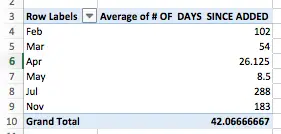
I produced this from your data using a Pivot Table. The basic steps were:
- Select the data
- Choose the option to Insert a Pivot Table using Date in the Rows section and Days Added in the Values section.
- Change the Days Added element from Sum (the default) to Average.
- Group the data in the Pivot Table rows by Month (and also by Year if your data spans multiple years).
- Done.
One extra thing that you'll need to do before you start with the spreadsheet you supplied. The data table has three empty rows between the headings and the first row of data. You'll need to delete those if you want the steps above to work, otherwise Excel may treat the first row of data as the headings in your PivotTable.
I hope this helps. Let me know if you have any further questions.
Regards
David
Are there row limits?
Internet was terrible last night so I am trying this again. I do multiple lookups on a column named search (list of surnames) the return is the full names in the second column of data. In a file with 27,000 rows this has worked great, even allowing me to list additional columns of information (C1, D1, etc.). When I increase the file to 59,000 rows my formula has the error #value!. Even with only the two columns search (surname) and FullNname in the data array Data B2:C59000. When I cut my data back to 20000 or 30000 rows it starts working again. Not sure where the break point is. Here is my formula:
=(INDEX(Data,SMALL(IF($B$1=Data,ROW(Search)-MIN(ROW(Search))+1,""),ROW(Sheet1!B1)),COLUMN(Sheet1!B1)))
Thanks for any advice you can offer.
Correct Row and Column return incorrect number value
My formula returns the correct Row number and I have the correct Column number however the value it returns is completely wrong. This is driving me nuts!! Any ideas??
Creating a report
I have a table with 39 columns and about 2400 rows that is going to keep growing. I need to be able to have a look up value for the customer name and have it pull all entries with this customer name along with 19 of the columns information onto a report. I was able to create an alternative report that looked up a specific sales Id and pull all the rows for the sales id but they were all in a row. =IFERROR(IF($D$7=$M17,INDEX('Asset Management Tracking'!$AE$4:$AE$2877,MATCH($D$7,'Asset Management Tracking'!$A$4:$A$2878,0)),""),"") I don't know how to get it to look up all values in the table and produce multiple rows of data.
Using this example on different worksheets
Hello, I'm trying to use your example to plug in an account on the first page and have all of the accounts contact information come up on that same page referencing the next page called 'Wholesalers'. All the data is on this Wholesalers page. I can't seem to get the formula to work as it keeps referencing the Sheet1 instead of the Wholesalers page in regards to the Row function. Also, the accounts are all listed in one cell on the Wholesalers worksheet and I need the formula to pull up all the contact information for a certain account when I put it in on the first page. There are multiple contacts per account. Basically I'm just trying to plug in the account and get all the account information on Sheet1. I'm pretty novice when it comes to Excel.
Any help would be greatly appreciated. Thanks!
Great Lesson -- Thank You
Great Lesson -- Thank You
Simply Superb!
This has been racking my brains for far too long! thanks for such a clear and easy to follow explanation.
Can't get it to work with data in a different location
Hi,
I found your exapmle and it seemed like it would be perfect. Thanks for putting it out there for us to learn!
I modifed it to work with my data but I can't get it to work. I can recreate your original example without any issue...here is the formula from tab 3 in my file.
=IF(ISERROR(INDEX($A$2:$C$7,SMALL(IF($A$2:$A$7=$A$9,ROW($A$2:$A$7)),ROW(1:1))-1,3)),"",INDEX($A$2:$C$7,SMALL(IF($A$2:$A$7=$A$9,ROW($A$2:$A$7)),ROW(1:1))-1,3))
However when I change it to fit my data with the following formula from the grower summary sheet in my file:
=(INDEX($M$2:$O$144,SMALL(IF($M$2:$M$144=$B$1,ROW ($M$2:$M$144)),ROW(1:1))-1,3)),INDEX($M$2:$O$144,SMALL(IF($M$2:$M$144= $B$1,ROW($M$2:$M$144)),ROW(1:1))-1,3)
It doesn't work. I was originally trying to pull the infomation for the grower summary sheet from the main sheet but that wasn't working either so I put the index info on the same sheet.
I'm attaching the file and hoping you can help me.
Adrienne
Index & Small formula issues
I am using this formula:
=IF(ISERROR(INDEX('ALL-BY JOB'!$A:$X,SMALL(IF('ALL-BY JOB'!$A$3:$A$681=A$1,ROW('ALL-BY JOB'!$A$3:$A$681)),ROW('ALL-BY JOB'!2:2))-1,2)),"",INDEX('ALL-BY JOB'!$A:$X,SMALL(IF('ALL-BY JOB'!$A$3:$A$681=A$1,ROW('ALL-BY JOB'!$A$3:$A$681)),ROW('ALL-BY JOB'!2:2))-1,2))
However, for any particular account, I may have 10 entries on the original tab of my spreadsheet "ALL-BY JOB" but only 9 appear on the final product. What am I missing?
Well Cool
Many thanks, I really appreciated 'Albert Ayler' and 'Beet'. Brilliant.
Look up reference
Hi,
I need to create a spreadsheet for quoting, using a look up list to find the item then the associated cost for that product and just can't get my head around it.
Sheet1 will be the quote form referring to Sheet two for pricing.
Please help!
Thanks
How to create formula to find out the data from other table?
All simple data have show on the simple file, table!B2 is the drop-dawn list with data validation to restrict the values from the sheet of table2!C3:C6, and how to create some formula on D2:E6 to find the related value from the sheet of table1?
How to Sum/Merge same values
hi, first of all thanks alot for the formula and particularly excellent way of narrating its each part to make us understand it easily.
i have used this code and its working perfectly, but i want to add a condition where it may add same type of values as exampled below:
Look up value is D2 = Bank
using ur formula it would show in my new sheet all the entries in Main sheet having Bank account in Colum A And result are as follows
Voucher No(Colum A) Dr (cOLUM B) Cr (cOLUM C)
1 500 Dr
2 200Dr
3 700 Dr
3 200Cr
4 100Dr
5 210 Dr
Now in above example voucher no 3 appeared twice, once dr and once cr, i want it to show it only once after rounding off the balance (700-200) 500 IN Dr feild
kindly guide me abt it
Regards
My formula wont work
My formula keeps giving me a #VALUE error, not sure what I am doing wrong as i have attempted to make it work multiple times.
I am having issue with final formula on partial match
I have worked my through the formulas and they all work great and this is exactly what I am looking for but the last formula for partial match works for first cell A11 in your example but A12 and all other cells I drag the formula down to show value for first hit. I am not sure what I am doing wrong. Like other examples second cell like A12 would show next hit that is a match on value in A9.
Thanks for any help..
I've updated the lesson to explain how to do this correctly.
Hi Kevin
Sorry - there wasn't enough explanation in the final example using partial matches. You can't copy and paste the formula from A11 to the cells below in this example. Instead, select all of the cells, click in the formula bar to start editing the formula (but don't change anything), and then enter the formula as an array formula. This will give the correct results as shown in my example.
I've updated the lesson to include these instructions.
I hope that helps - post back here if you are still stuck.
Returning Values Less Than with if Statement
Hi.
First, I want to thank you for this lesson. it is easy to follow, well explained and quite useful.
I have the base formula working as you show it with no problem. However, I have additional needs in a formula. I want to return values that are less than a certain time. the formula returns that information, however it is looking at all of the items that match and then, in the row it matches, it places the data in that row.
For example. If it matches the 20th instance, then it will place it in row 20, leaving the other 19 rows above it blank.
Is there a way to make it return the values as it finds the correct one, rather than going by each one and checking it off the list and moving to the next row?
Please see attached file for more details.
Thank you
First results row duplicated
This is great! I'm using it to return all orders that are due on a date the user selects in a calendar. The problem I'm having is, that the first results row is being duplicated. If my table data starts in row 6, and there are 6 matching rows (6-11), the equivalent of your formula ({=SMALL(IF($A$2:$A$6=$A$9,ROW($A$2:$A$6)),ROW(1:1))}) correctly shows that rows 6-11 are being returned. All subsequent formulas result in #NUM as expected.
However, the results of the INDEX function to find the Crop value returns results from table row 6 for the first formula, but then returns the same results for the next row (although the returned row number shows "7" as expected), then results from row 7 in what should be row 8, etc. So after the first duplicate, the results are always 1 row behind. But what should be the last match results in #NUM.
Hope this makes sense, but please take a look at the attached for a better explanation.
Thanks!
Re.: First results row duplicated
Never mind, I found my problem
Use INDEX to lookup multiple values in a list
Hi, I just saw your lesson about index for multiple values in a list. I found it to be very good and useful for my problem. Clearly am new in this but working with reports has submitted me to excel very fast and some time I need to do report using a huge data's. in my problem I have a list of coils and respectively dates used, coil n's and so on, the thing is that the coils nr are different but the weight can be the same. what I need is to use index for multiple values that will return for example the list of all coils( remember, the weights can be same for different coils nr) used in a day X.
Returning Multiple Values in One Cell
In your given scenario above, is there anyway to return all the matched items in one cell? By this I mean, when we have duplicate look up values, ID H240 in your example, can excel return all the results in just one cell instead of having to do it by individual rows/cells?
Using multiple arguments to return a row number
Hello,
This function almost works perfectly for me but I'd like to be able to use multiple arguments to return a row number. So ideally, the first part would look something like: SMALL(IFS('Drill Log'!D:D=Mon!$B$8,ROW('Drill Log'!$D:$D),'Drill Log'!C:C=Mon!$H$8,ROW('Drill Log'!$C:$C),ROW(1:1). Basically just using two different criteria and having the small function return the first instance. Using the "ifs" function was just the first thing I tried, if anyone has a better way I'd be all ears.
Thanks in advance!
-Matt
Solution?
Hi mate, have you had any succes in finding a solution for this? Could really need the help :)
Need help to get the results on one row
Need help to get the results to be on one row instead of downwards in a colums.
Exampel:
1 a
2 b
3 a
4 b
result after using the formula, when looking for a:
1
3
Need the result to be like:
1 3 ...
Hope someone can help me with explain how this is done.
In advance thank you.
my question fall out
som mye question was:
I nedd the result to be in a row instead of a colum.
exampel:
1 a
2 b
3 a
4 b
Refult after using the formula in sherch of a:
1
3
But in need the result to be in one row after each other
1 3
Hope that someone can help me withe excplaning how to do this.
In advance thanke you.
Column
You just need to change "ROW" to "COLUMN" and "1:1" to "A:A"
=IF(ISERROR(INDEX($A$2:$C$7,SMALL(IF($A$2:$A$7=$A$9,COLUMN($A$2:$A$7)),COLUMN(A:A))-1,3)),"",INDEX($A$2:$C$7,SMALL(IF($A$2:$A$7=$A$9,COLUMN($A$2:$A$7)),COLUMN(A:A))-1,3))
Changing formula in adjacent cell
I am trying to change the formula in D17 to -1,4 to capture the age column. When I enter it there it changes it back to -1,2 as is shown in C17. Worked great in B17 capturing the day.
You're amazing
This is great! I had a formula that did this that I'd found from somewhere else, but when I needed to make some changes the thing broke! This solution is much more elegant and I feel like I finally understand its behavior. Thanks a million!
How can I have all matches display in one cell?
How can I have all matches display in one cell instead of one row per match?
Thanks!
Thank you for this: this helped solve a problem I'd been trying to find a solution to for a few days. Had tried this method from a tutorial I'd found elsewhere, but this one explained it so much better, and helped to get it working. Explaining the SMALL function in isolation was particularly useful!
Using two variable in an If statement
The formula you have provided worked great as a foundation for what i am trying to accomplish but I am struggling in adding an additional If statement to check for a different variable.I need to check index off of a date but only for rows that contain one of two values. Any suggestions?
What if I move in columns not in rows
Hi,
The formula works perfect if I drag down in a row, then as you showed it changed ROW(1:1) to ROW(2:2) etc. But if I want to find multiple values which are in a row and fill them as a column then dragging does not work. ROW(1:1) stays the same. Of course I can add one more step finding values and filling in a row and then transposing them, but I would like to skip this step. Do you think it is possible?
Awesome!
This worked so well. I was looking for a way to do a "reverse countif" kind of thing and this does it. Thank you!
I couldn't get this to work
I tried the formula but I must have messed it up somehow. Row 1 works great (same as a vlookup) but row 2 doesn't work. Here are the 2 formulas
=INDEX('[2019-01 liab 020519.xlsx]Sheet2'!$V:$V,SMALL(IF(A2='[2019-01 liab 020519.xlsx]Sheet2'!$C:$C,ROW('[2019-01 liab 020519.xlsx]Sheet2'!$C:$C)-ROW('[2019-01 liab 020519.xlsx]Sheet2'!$C$3)+1),ROW(1:1)))
=INDEX('[2019-01 liab 020519.xlsx]Sheet2'!$V:$V,SMALL(IF(A3='[2019-01 liab 020519.xlsx]Sheet2'!$C:$C,ROW('[2019-01 liab 020519.xlsx]Sheet2'!$C:$C)-ROW('[2019-01 liab 020519.xlsx]Sheet2'!$C$3)+1),ROW(2:2)))
There are 2 numbers that should match but row 2 is coming up #NUM!
Multiple criteria
Excellent lesson, thank you. Is it possible to search through a range instead of a single criteria in A9? I have tried numerous ways (A:A, Table1, "xxx","xxx", etc) but each time I get a blank result.
Best Explanation
This is the clearest explanation of this issue you'll find online. Kudos to you.
How to copy and paste the formula (not the partial formula)?
Thank you for your time and this formula is awesome!!!
Now, how may I reuse this formula in vertical order once all values have been found?
I noticed that, I need to change the ROW(#:#) to start with 1:1 after every criteria, but how may I avoid changing the syntax after I enter a new searchable criteria?
For example, table:
-Column A, searchable criteria, Client ID
-Column B, all values found, Crop
How to copy the same formula in from B4 to B5 and there after every time I enter a new client ID?
Or maybe I can add to the formula if error/blank then next....
"A" "B"
1) Client ID Crop
2) H240 Beans
3) Corn
4) Hops
5) W869 Corn
6) Beats
7) X323 Hops
8) N503 Beans
My work around is, copy formula from B4 into B5, change syntax, ROW(4:4) to ROW(1:1). Then press, Ctrl + Shift + Enter. But I do not wan to do the same for all 100 + client's ID.
Column Function
Hi...what if my data's are arranged horizontally. I know i can transpose this and use the above formula....but still....i tried to apply the formula horizontally....its working for the first cell.....i replaced ROW function with COLUMN function...however its not working for subsequent cells. Can you help out on this??
Thank you
Can this formula be used with multiple criterias?
Hello,
Using the same fundamentals, is there a way to add more criteria? I have a unique identifier for each individual, but I would also like to narrow the results down as of location.
This is the formula I'm using, but I don't know where or how to add a second criterion:
{=IF(ISERROR(INDEX(STU415Course,SMALL(IF(STU415SAIS=$B9,ROW(STU415SAIS)),ROW($1:$1)))),"",INDEX(STU415Course,SMALL(IF(STU415SAIS=$B9,ROW(STU415SAIS)),ROW($1:$1))))}
I titled location as "STU415School".
Best regards.
index examples
i this example we got the crop values in a11,12,13
how can we have these values in a11 as a data list
index match multiple values
i have a timetabel for several people and i wish to return a date value depending on name and (if possible by months) but i managed to make it only for one column, not depending on the name. may be i just overcomplicated it.
thank you in advance
index match multiple values
i have a timetabel for several people and i wish to return a date value depending on name and (if possible by months) but i managed to make it only for one column, not depending on the name. may be i just overcomplicated it.
thank you in advance
I cannot figure a way to add a function to my spreadsheet - essentially what I want to happen is that when a person enters a year in cell c12, the value of cell c14 changes to the dollar amount of the package for that year - which I have in a table on the same sheet. I tried to get this to work with vlookup but have had no joy. I want to set the sheet up to automatically calculate a range of things with minimal input from users (and decreased errors as a result). If they know the year then I would rather have the sheet automatically populate with the approprate dollar value (which my team updates regularly based on indexation and cost changes).
Any advice would be much appreciated!
Cheers
Michael
Year Average cost
2013/14 $34,969
2014/15 $36,354
2015/16 $37,793
2016/17 $39,290
2017/18 $40,846
2018/19 $42,464
2019/20 $44,145
2020/21 $45,894
2021/22 $47,711
2022/23 $49,601
2023/24 $51,565