Using multiple IF statements in Excel
The IF() function in Excel allows you to evaluate a situation which has two possible outcomes (e.g. sales are greater than $1000) and calculate a different value for each outcome. However, sometimes you need to work with situations where there are more than two possible outcomes. That's where multiple, or nested, IF functions come in handy. In this tutorial we'll cover how to use nested IF functions to calculate sales commission for a team of sales people, given a range of different commission rates.
This lesson assumes you are already familiar with the IF function. If you aren't, you can learn how to use IF statements here.
Remember that the IF function works by evaluating a logical test - a calculation which can only be TRUE or FALSE, or 1 or 0. It then includes a calculation to perform if the logical test is TRUE, and another calculation if it is FALSE.
Nested IF functions work by replacing one or both of the TRUE/FALSE calculations with another IF function.
Calculating commission for a sales team based on monthly sales
Imagine you have a sales team of five people, and you need to calculate their commission for the month based on their sales figures.
- You put the data into the following table:
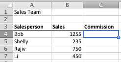
- Your commission plan works as follows:
- If someone sells less than $400 in a month, they get 7% commission.
- For sales between $400 and $750, they get 10% commission.
- For sales between $750 and $1000, they get 12.5%
- For sales over $1000, they get 16%
- Rather than calculate each of these commission figures individually, you decide to use a nested IF formula instead. The logical tests you would use in this case are these:
- Is commission less than $400? If TRUE, then calculate commission.
- If FALSE, then is commission less than $750? If TRUE then calculate commission.
- If FALSE, then is commission less than $1000? If TRUE then calculate commission.
- If FALSE, then calculate commission (because it must be more than $1000 - we don't need to do another logical test for this).
- The formula to represent this to calculate commission for Bob looks like this (I've highlighted the logical tests in bold to help you understand now the formula is put together:
=IF(B4<400,B4*7%,IF(B4<750,B4*10%,IF(B4<1000,B4*12.5%,B4*16%))) - This formula can be confusing the first time you look at it. Let me run through it again.
- The logical test in the first IF statement checks if the sales figure in B4 is less than $400. If it is, it calculates commission at 7% and stops calculating. Otherwise, it must be greater than or equal to $400, so we move on to the next IF statement.
- The logical test in the second IF statement checks if the sales figure in B4 is less than $750. We already know it must be more than $400 or we wouldn't have got to this point. If it is less than $750, it calculates commission at 10%. Otherwise it must be greater than or equal to $750, so we move on to the next IF statement.
- The logical test in the third and final IF statement checks if the sales figure in B4 is less than $1000. If it is, it calculates commission at 12.5%. Otherwise, it must be greater than or equal to $1000, so it calculates commission at 16%. At this point there are no more IF statements, no more logical tests we need to do, and we have our answer.
- Here's how our spreadsheet example looks once the formula has been entered into the Commission column. I've put the formula for each sales person in the cell next to the commission calculation so you can see how it looks:
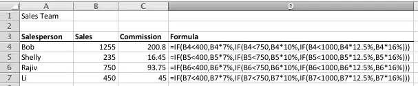
- Check Rajiv's commission figure in the table above. Rajiv sold $750 in the month, which is right on the threshold between 10% and 12.5%. What commission does he get? He actually gets 12.5% because the formula checks whether his sales were less than $750, not less than or equal to $750. That means he receives commission at 12.5%. So it's important to pay attention to how you construct your logical tests.
Some things to remember when using nested IF functions
Nested IF functions are very powerful, but there are some things to consider before you dive in and start using them.
- As you can see from the commission formula above, using nested IF statements gets complicated quite quickly. Trying to decipher this takes a moment or two, especially if you haven't looked at the spreadsheet in a while.
- Making changes is also challenging - imagine if you decided to introduce another commission threshold of $850. You'd need to add another IF function into the formula.
- You can have up to 64 IF functions nested in a formula in Excel 2007, 2010 and Excel 2013. Excel 2003 only supported 7 IF functions in one formula. That said, if I find myself needing more than 10 I start considering other approaches to my problem - managing that many IF functions in one formula quickly gets complicated, never mind if you have to manage 20, 30, 40 or more.
- The VLOOKUP function can sometimes be a better solution in a scenario like this. You can see a really good example of where you should learn how the VLOOKUP function works in one of the comments below.
- That's not to say that VLOOKUP is automatically a better solution:
- A commission spreadsheet like the one shown above is a good example where using VLOOKUP would be a better approach.
- However, if you needed to use different calculations depending on the outcome of each logical test, then nested IF statements may well be a a better way to go.
- An example might be where sales people who exceed $1000 in sales also get a bonus of $100. The formula would then look like the following, which is not so easy (although not impossible) to do with a VLOOKUP function:
=IF(B4<400,B4*7%,IF(B4<750,B4*10%,IF(B4<1000,B4*12.5%,B4*16%+100)))
Finally, I've supplied a copy of the spreadsheet I used for the example above. You can download it here.
Our Comment Policy.
We welcome your comments and questions about this lesson. We don't welcome spam. Our readers get a lot of value out of the comments and answers on our lessons and spam hurts that experience. Our spam filter is pretty good at stopping bots from posting spam, and our admins are quick to delete spam that does get through. We know that bots don't read messages like this, but there are people out there who manually post spam. I repeat - we delete all spam, and if we see repeated posts from a given IP address, we'll block the IP address. So don't waste your time, or ours. One other point to note - if you post a link in your comment, it will automatically be deleted.
Comments on this lesson
Nested IF statement
Use this formula IF(E1<5999,150,IF(E1<60007999,300,IF(E1<800011999,400,"Some stmnt here")))
which use the IF statement with the Cell reference and check the last statement.
Make sure that the number of
Make sure that the number of If's you use are the same in terms of number with the number of closing bracket
help ! i have tried multiple diff formulas and nothing
min is 75 $ - 0.55 per kg - +45 0.55-+1000.60- +500 0.70 - +500 0.75- +1000 0.85.- +2000 0.90
gross weight is 100
2000
3000
234
122
1222
300
6000
formula
=+IF(AND(C13<5999),150,IF(AND(C13>=6000,C13<=7999),300,IF(AND(C13>=8000,C13<=11999),400,IF(AND(C13>=12000,C13<=14999),500)))) and so on
Thank you IF(AND(),)
This is really helpful, luckily i come across your post about IF(AND(),) condition.... Thanks a lot.
How to combine multiple IF Conditions
I want to calculate %age for the values located at different cells.
Min to mean% and mean to Max%, If the cell value is below mean it should take one formula and if the cell value is above mean it should take another formula.Tried below formula but could not get the result, pl advise
IF($V3<AA3,($V3/AA3*100-100),IF(AA3<$V3,($V3/AA3*100-100)))
USING THE FOLLOWING
USING THE FOLLOWING INFORMATION, PLEASE PROVIDE ME THE CORRECT FORMULA IN EXCEL.
Gross Monthly Earnings Amount to be contributed
Php 8,999.99 and below Php 100.00
9,000.00-9,999.99 112.50
10,000.00-11,999.99 125.00
11,000.00-11,999.99 137.50
etc.
Thank you in advance.
Use a VLOOKUP table instead of multiple IF statements
Hi Felix
Whilst you can get the result you want using multiple IF statements in a formula, I recommend you look at using a VLOOKUP function instead. You'll find it a lot easier, and more flexible if you need to change it later. You can learn about the VLOOKUP function here.
David
@Samuel Wainaina
Use VLOOKUP with true option for your range
its much easier than using IF function
If Statement
Need help. wrote following If statement, but all it gets me is True or false.
=IF(D5>89%,"A",If D5>79%,"B", IfD5>69%,"C")))))
Tryding to equate the percentages to a letter grade
Try without the % sign
I'd try this:
=if(d5>.89,"A",if(D5>.79,"B",if(d5>.69,"C","Fail")))
Note how I used the numeric value rather than a % value.
The example you gave was also missing the () in the correct places. Also, if you don't have a value for "Fail" as shown in my example, it will show FALSE as the result in the cell. You could put "" if you want the cell to be empty if the grade is not above 69%.
Also consider whether you should use >=.9 rather than >.89 - this will be more accurate if 90% is required for an A grade (your example would assign an A to a grade of 89.5%.
You can use the percent
You can use the percent symbols your missing the parenthesis after your IF
I don't even know where to start..
First, I would like to say thank you for your terrific lessons and taking the time to respond to the questions your visitors ask; it is very kind and helpful.
I hope you can help me, as I don't even know where to start. I am to create a formula in which the changes will be consistent throughout. Here is an example of what I am trying to achieve:
I have a dollar amount in cell M2. This dollar amount is sales numbers.
Column N is titled Blue Shirts, O is Red Shirts, P is Green Shirts, Q is Pink Shirts and R is Orange Shirts.
There is a bonus for each shirt the salesmen sells; the bonus is also determined by their total sales.
If the salesrep sells less than 750, there is no sales volume bonus. If they sell between 751 and 1,200 there is a 2% bonus; between 1,201 and 2,000 there is a 3% bonus; if they sell between 2,000 and 2,500 there is a 4% bonus, Etc. Etc.
If they sell a Blue shirt, the bonus is 0%, Red shirts is a 2% bonus, Green is a 1.3% bonus, pink is a 1.3% bonus and orange is a 1.3% bonus. ** This bonus will be on top of the sales volume bonus!
Each column for the color of shirts sold has an ‘X’ marking if they sold that color.
Is it possible to create a formula using an IF formula which will allow me to calculate the sales volume bonus AND the bonus for color of shirts sold so it is all tied in together?
I hope this makes sense, it is very hard to explain! This is the formula I have so far for just calculating the sales volume bonus (something is not working right, I am having a hard time making it consistent all the way down the rows):
=IF(M2<400000,M2*Data!$C$3,IF(M2<400001,M2*'Volume Bonus'!$C$5,IF(M2<600001,M2*'Volume Bonus'!$C$6,IF(M2<900001,M2*'Volume Bonus'!$C$7,IF(M2<1200001,M2*'Volume Bonus'!$C$8,IF(M2>1800001,M2*'Volume Bonus'!$C$9))))))
I thank you so much in advance for even taking the time to look at this problem, I sure hope you can help!
I should have been more clear..
For an example, the end result will tell me if the salesrep sold 450, they receive a 2% bonus; they also sold a red shirt and a orange shirt (which makes it a total of 3.3% bonus. How much is the total bonus given?
This will need to be done for a few hundred rows. Each column for the shirt colors have an X in the row to indicate if they sold that color...
Complicated Sales Commission Calculation (with download)
Hi Kristin
What I love about Excel is that there are many ways to skin this cat. Here's one which doesn't even use any IF functions (and stays considerably less complicated as a result).
First, let me show you how I interpreted your scenario:

I've calculated the Sales and Shirt bonuses in two separate columns, but the formulas could easily be combined into the same column once you've got it working.
I've also made an assumption that if some sells <750 then they get no bonus at all. That's why sales person B and C get nothing even though they both sold red shirts. It's easy to remove that assumption from the example, as you'll see.
I also created two separate tables to contain the threshold sales values and the commissions for each colour so that I can keep my formulas simple. I'd normally put them on a separate sheet to the sales data, but for this example they're on the same sheet:
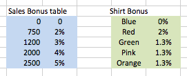
Note that I have named each of the cells in the Shirt Bonus table so I can refer to the formulas by name. I won't cover how to do that here, but will come back to it in another lesson. Suffice to say that the cell containing the bonus for Blue is called, well, Blue. Naming a cell lets me refer to it by name in a formula rather than by using $F$14.
I then created the formula to calculate the sales commission based on actual sales (Sales Bonus). For this, I used a VLOOKUP() function to compare the sales with the values in the Sales Bonus Table. Here's the formula for sales person A:
=VLOOKUP(B2,$B$14:$C$18,2,1)
You can learn more about how to use VLOOKUP here.
I calculated the Shirt Bonus like this:
=((C2="X")*Blue+(D2="X")*Red+(E2="X")*Green+(F2="X")*Pink+(G2="X")*Orange)*(B2>750)
As I promised, no IF functions at all. Here's how this works.
- It looks at the value in C2 (the Blue column) to determine if it contains "X".
- If it does, the value of (C2="X") is returned as TRUE, or 1.
- If it doesn't, the value of (C2="X") is returned as FALSE, or 0.
- I then multiply the result by the value in Blue. If it doesn't contain "X", then the result will be multiplied by 0 which gives 0. Otherwise it's multiplied by 1, which gives whatever is in Blue (or Red, and so on)
- I repeat this for each column.
- Finally, I then look at the sales value to determine if it is >750. Again, the result is either 1 or 0. I multiply this by the rest of the formula. So if the sales value is <750, the result of the whole calculation is 0, otherwise the value is allowed to stand as calculated.
If you want to pay a bonus on shirt sales regardless of the $ value of sales, simply change this formula like so:
=(C2="X")*Blue+(D2="X")*Red+(E2="X")*Green+(F2="X")*Pink+(G2="X")*Orange
Having done this, I then add the two commission values together in column J, and calculate the $ bonus in column K. Once again, you could combine all of these into a single formula if you want.
The only shortcoming of this approach is the need for the two tables for Sales and Shirt bonuses. However, while it might be a shortcoming, it also gives you greater flexibility to extend the number of shirt colours in future, and also to change the threshold sales levels and related commission amounts.
Hopefully this gives you the result you're looking for - if not, please let me know!
I've attached my worked example here for you to dissect and re-use as you see fit. If you'd like more help, feel free to get in touch directly via the contact form.
David
if function with 4 arguments
please help me with my problem
in attendance matter
scenario:
if les than 8:30:00 am it will appear PRESENT
if greater than 8:31:00 am it will appear LATE
then if 9:01:00 am it will appear is HALFDAY
den if absent it will appear ABSENT
hope you can help me with this problem
In Between
How would you do in between ranges like this:
=IF(G4<100,100-G4,IF(G4>100<105,105-G4,IF(G4>105<115,115-G4,,IF(G4>115<125,125-G4,)))
Using IF on ranges
There are three ways to achieve this.
Option 1
In your example, you are doing this:
If G4 < 100 then the result is 100-G4. If G4 is not < 100, then move on to the next IF statement.
You have then tried to use G4>100<105, i.e. if G4 is more than 100 but less than 105. The thing to remember is that we already know that G4 is greater than 100, because it failed the test in the first IF statement. We wouldn't even be using the second IF statement if it had passed that test. So your function could look like this:
=IF(G4<100,100-G4,IF(G4<105,105-G4,IF(G4<115,115-G4,IF(G4<125,125-G4))))
Remember that each IF statement is only evaluated if the previous IF statement tested FALSE.
Bear in mind that the way I've written this function assumes that if G4=100, then the calculation will be 105-G4. Is that what you wanted? If not (i.e. if G4=100, then calculate 100-G4) then you should change each IF statement to <=, rather than <.
Option 2
The other option you have is to use the AND function as well as the IF function, like this:
=IF(G4<100,100-G4,IF(AND(G4>=100,G4<105),105-G4,IF(AND(G4>=105,G4<115),115-G4,IF(AND(G4>=115,G4<125),125-G4))))
This is longer, more complicated, but allows for a situation where you need to be specific about the parameters of the test you're performing. Note that the AND function requires that both statements be TRUE for the AND test to return TRUE to the IF function. As a side note, you could also use the OR function here if only one of the statements needed to be true.
Again, notice that I've used the <= symbol in each AND - if I hadn't, the formula would not always have returned the correct result.
Option 3
You can also use a VLOOKUP function rather than an IF function. I'd be inclined to take this option since it allows you to create a table of threshold values that the VLOOKUP function references, and you can change or add to those values at any time without having to rework your formula.
You can read more about the VLOOKUP function here (opens in a new tab).
Thank you! I test both, I
Thank you!
I test both, I wanted to avoid doing a vlookup to another table, but that is a great option. Both option 1 and 2 work, I went with option 2 and modified it to handle %.
=IF($G31<1,1-$G31,IF(AND($G31>=1,$G31<1.05),1.05-$G31,IF(AND($G31>=1.05,$G31<1.15),1.15-$G31,
IF(AND($G31>=1.15,$G31<1.25),1.25-$G31,"Achieved Top Tier %"))))
I really appreciate you taking the time to respond and so quickly!!!
Another Choice for Zero
Hi! Please can you help me? I need an IF equation for an answer of zero that returns different text than a false response. Thanks!
Situation (a) Plan is more than or equal to Actual = answer of Well Done!
Situation (b) Plan is less than Actual = answer of Oops...Over!
Situation (c) Plan=zero and Actual=zero = answer is no text at all.
=IF text question
can you help me please
i need a formula that will return a text initial based on the text in another cell;
for instance
if cell C20 contains "JAIL" (w/out quotations) then T20 will show "J" (w/out quotations)
i have been working on this for some time and can only get it to return #name?
thanking you in advance!!!
laura
THANK YOU!!! after just a few
THANK YOU!!! after just a few minutes of searching your lessons i figured it out..
=IF(C20="JAIL","J","")
and it was simple as i thought it would be.. i just couldn't see the forest for the trees i suppose :)
laura
how to use If and() & 0r() fuction
which funtion is used and how to get greatest number among them which can be written as e.g "first NO is greatest".plz solve my problem
Help
Hi,
I wonder if you can help. I am trying to Apple this formula for about 90 players using VB how do I do so?
=IF(G2:G15=AR4,AS4)
What I need to do is nested IF Statements however Excel only allows 7, so I thought maybe I could create a function in VB Excel.
What I need i to do is auto populate a cell A with if Cell B (Player Name) matches Cell C (Player Names)
Ok so to put it in pseudo code:
IF( Player Name entered in Cell A is = Player name on a list of players in Cell B, Take that Players Position in Cell C and put it in his Postion Column in Cell D)
E.G. I enter Tom, it looks in Cell B, if Tom Exists in Cell B, it looks for his Playing Position e.g. Defender and auto populates his Position in Cell D so resulting in it tell me Tom is a Defender.
I now want that to do so for any given cell in A.
Hope I make sense, and I hope you can help. Thanks in advance
Hi I have a similar scenario
Hi
I have a similar scenario but it has an accumulation on rows so will try to explain.
I have a sales threshold of £10,000 before i earn commision, in my spreadsheet i need to record products sold and the order value. To help with the formula i have created two columns, "Order Value" and "Claimable Value". So for instance in row one i sell something for £8,000 so enter this in to the "Order Value" column, in the next column "Claimable Value" i used the formula =IF(B2<(A1),"0",SUM(B2-(A1))). So in A1 i enter my threshold of £10,000, then in Cell B2 i enter £8,000 (Order Value) so the value then returned in C2 (Claimable Value) is £0....perfect. If i changed the "Order Value" to £12,000 in B2 then C2 returns £2,000....perfect as i know i can then apply a percentage commision to C2.
Now for my problem, when i move to the next line i can't figure out the cummulative formula to take in to account multiple lines. In my sheet i have a potential for 30 lines, as soon as i get over £10,000 in any line i want the "C" column to show the amount. So stick with the first example above in B2 i enter £8,000 so C2 returns £0, then on the row below in B3 i sell something for £4,000 because B2 & B3 exceed A1 by £2,000 (£10,000) i need the calculation to enter £2,000 in to C3. I could then move to the next line and enter £3,000 into B4, but this time i have already exceed £10,000, the calculation has given me the value in C3 but with this new sale i need to discount that as i am already over my threshold so get paid on the £3,000 in B4 so need this entered in to C4. Reason being each line has the potential to get paid at a different percentage which i enter else where so each distinct row needs to return it's value taking in to account the previous row and the threshold, to say i am stuck is an understatement.
As i said the formula above works perfectly for one row but expanding that to the rest is getting impossible, can you help?
Calculate sales as a running total
It looks like there are a couple of things you need to do here.
First, you should use an absolute reference to A1 in your formulas. In the example you used for C2, it would look like this:
=IF(B2<$A$1,"0",SUM(B2-$A$1))
The $ signs make the reference to A1 absolute. Not matter where you copy this formula within your spreadsheet, this formula will always refer to A1.Then, when you copy the formula in C2 down to C3, the formula in C3 will look like this:
=IF(B3<$A$1,"0",SUM(B3-$A$1))
Notice that the formula still refers to A1. Notice also that I removed the brackets you had around A1 in your example, since they aren't needed, and removing them simplifies the formula.
However, the real problem you've got is that this formula doesn't take account of additional sales in subsequent lines. Therefore, the formula you really need in C2 is one which calculates a running total of your sales, like this:
=IF(SUM($B$2:B2)<$A$1,"0",SUM($B$2:B2)-$A$1))
In both cases, the SUM function here will add up all the values between B2 and B2. This may seem odd, but it makes more sense when you look at this formula after copying and pasting it into C3:
=IF(SUM($B$2:B3)<$A$1,"0",SUM($B$2:B3)-$A$1))
Now the SUM function is calculating the sum of all the values between B2 and B3, i.e. your accumulated sales for those two lines. Therefore, if the cumulative total remains below the threshold value in A1, your commission will be 0. Otherwise, the commissionable amount will be the cumulative total minus the threshold value.
Let me know how you get on with this solution. You can read more about absolute and relative references here, and more about calculating a running total here. Both of these links will open in a new window. If you're still stuck, either post your questions here or contact me directly.
IF MULTIARGUMENTS
=IF(Sheet1!F3<="8:30:00 AM","PRESENT",IF(Sheet1!F3>="8:31:00 AM","LATE",IF(Sheet1!F3>="9:01:00 AM","HALFDAY",IF(Sheet1!F3="","ABSENT"))))
Please help me with this formula the 3rd and 4th arguments does not work
only the first and second argument work
MULTIPLE IF - WITH ADDITION
I have a complex formula and need to consider variables AND addition. Here's my scenario.
- My users will determine the variables by marking 'Y' or 'N' on each of 8 store segments
- My formula must take each of the 8 criteria into consideration and pass that column by (if it's an 'N') or use the field for calculation if it's marked 'Y'
- In some scenarios, ALL 8 store segments could be in selected
Here's my formula, and it's not performing as intended:
=IF($M8="y",$M12*V$9,IF($M8="N",0)+IF($N8="y",$N12*V$9,IF($N8="N",0))
+IF($O8="y",$O12*V$9,IF($O8="N",0)+IF($P8="y",$P12*V$9,IF($P8="N",0)
+IF($Q8="y",$Q12*V$9,IF($Q8="N",0)+IF($R8="y",$R12*V$9,IF($R8="N",0)
+IF($S8="y",$S12*V$9,IF($S8="N",0)+IF($T8="y",$T12*V$9,IF($T8="N",0))))))))
To simplify for your reference, here's two segments of the formula:
=IF($M8="y",$M12*V$9,IF($M8="N",0)+IF($N8="y",$N12*V$9,IF($N8="N",0))
M8 denotes the first store segment
M12 denotes distribution centers n8 denotes the second store segment
V9 denotes the number of pieces per location
My question is this? How can I ADD the IF's together? A simple SUMIF won't work as I need the individual IF statements to function independently, then add the results together. HELP!
Any suggestions?
Try using a logical test on each criteria
My first thought is you probably don't even need to use the IF function for this scenario. I would try something like this:
=($M12*V$9*($M8="Y"))+($N12*V$9*($N8="Y"))+etc
What you'll find is that ($M8="Y") will evaluate to TRUE if M8 contains "Y" and FALSE if M8 doesn't contain "Y". In Excel, TRUE=1 and FALSE=0. So each segment in the formula will be multiplied by 1 or 0 depending on whether the check cell contains "Y". Those segments that don' t have "Y" will therefore be calculated as 0, and ignored in the final total.
If you want to idiot-proof this a little, you could allow for different inputs in M8 by replacing ($M8="Y") in the formula with the following:
(OR($M8="Y"),($M8="Yes"),($M8="y")))
This will ensure the formula works for a variety of inputs. The OR statement will evaluate each logical test within it separately (you can have as many as you like). If any of the tests are true, then the OR function will return TRUE. If all of them are not true, then the OR statement will return FALSE.
Hopefully this helps - if not, please let me know.
Help
Hi all,
i need to create a formula in excel sheet like:
if there is many type of cell like numeric and alphabet then how i create a multiple IF condition formula in sheet for exaple
if
H then H
if
W then W
if
CL then CL
if
Time 8:15 then P
kindly help
Checking if a cell contains text or numbers
It depends whether you want to test for specific text values, like H, W, CL, or whether you want to have one set of tests if the value is text, otherwise another set of tests if the value is a number (time is stored as a number in Excel).
You can use the ISTEXT() function to check whether a cell contains text. It will return TRUE if the value in the cell is a text value, and false if it is a number. This is a useful function if you have imported some data into a spreadsheet and need to check whether numbers have been imported as numbers or text values.
For example:
=IF(ISTEXT(A1),value_if_true,value_if_false)
The value_if_true and value_if_false would each be another IF statement, depending on what you want.
In terms of testing whether a value contains a certain time, you will need to use the TIMEVALUE() function.
For example, let's assume you've entered a time into cell A2 by typing 8:15 directly into the cell. Excel will recognise this as a time and store it as a number, but format it as a time.
Your IF function would then look like this:
=IF(TIMEVALUE("8:15")=A2,value_if_true, value_if_false)
Note that if you wanted to use 8:15pm, you would need to either enter the time as "20:15" or "8:15 PM".
Hi,
Hi,
Kindly help me to create formula for the below table:
achvmnt target %incentive
<90 0
90-99% 50%
100% 100%
101,102…199% 101,102…199%
200 &> 200% 200%
if the acheivement is < 90% i should get 0 as the incentive % if the acheivement ranges from 90-99% incentive% should automatically show 50%,if it ranges from 101% to199% -incentive % should be 101,102 means 102 like that it should follow if the incentive acheived by employee is more than 200% it should restricted to 200%
calculate income tax
kindly help me to create a formula:
i need to crate a calculator of income tax
if income <=200000 no tax
if income >200000 to 500000 10% tax
if income >500000 to 1000000 20% tax
if income >1000000 then 30% tax
i want it to be created in nested if .
Calculating Income Tax
Hi Tarun
This is a fairly simple scenario which a formula containing nested IF statements will handle easily:
Let's assume that the income amount is in cell A1:
=IF(A1<=200000,0,IF(A1<500000,10%,IF(A1<=1000000,20%,30%)))
This formula will calculate the amount of tax. To calculate the tax amount, you could use this version of the formula instead:
=IF(A1<=200000,0,IF(A1<500000,A1*10%,IF(A1<=1000000,A1*20%,A1*30%)))
I hope this helps!
Regards
David
Calculating income tax - response
Hi - I'm not sure this works. I was hoping that it would as it would solve a problem for me. In the example a value for A1 of 300,000 would return a tax payment of 30,000 (10%) but it should return 10,000. The first 200,000 is tax free so the 10% rate only applies to that portion of the value of A1 that is over the tax free threshold. I am trying (and failing) to structure a commission scheme on the same basis i.e. nothing is paid until a threshold of 100,000 is reached, the next 50,000 earn 10%, the next 50,000 15% - but the first 100,000 do not count so earnings of 200,000 earn 12,500 (50,000 * 10% + 50,000 * 15%). Can you suggest how to do this?
If Function using progressive tax and ranges
Hi I am having problems combining the following if functions into one formula:
=if(B19>=0,C7*15)
=IF(B7>50000,7500+(75000-50000)*0.25)
=IF(B7>75000,13750+(100000-75000)*0.34)
=IF(B7>100000,22250+(335000-100000)*0.39)
=IF(B7>335000,113900+(10000000-335000)*0.34)
=IF(B7>10000000,3400000+(15000000-10000000)*0.35)
=IF(B7>15000000,5150000+(18333333-15000000)*0.38)
For example, if some has income of 100,000. I want to calculate the tax.
So the first range is taxable income over $0, but not over $50,000 must pay 15% on for any amount over $0. Then the next range is taxable income over $50,000 but not over $75,000 must pay $7,500 plus 25% on income over $50,000 and so on and so forth.
Please help me! I have a difficult time combining the formulas. Thank you!!
I TAX
DEAR FRIEND,
THIS MAY HELP YOU.
Calculating incentives
Hi Priyanka
I've just posted a response to another comment directly below this one which looks at a very similar sales commission example. You should be able to use that example as the basis for solving your problem.
I would also recommend you consider using a VLOOKUP function instead. Your incentive table is fairly complicated and (I suspect) subject to change over time. Keeping the table in a separate location on the spreadsheet and referring to it from a VLOOKUP function will make it much easier to change the contents of the incentive table. You can read our VLOOKUP lesson here (opens in a new tab).
Regards
David
Help with Nested IF/AND with text Evals included
Hi!
I have a formula I have been working on for awhile now and I am close but not quite there and hoping you can help.
I have the following table example.
Level # Shifts Y or N?
A 3.1
AG 1.5
AD 0
P 3.5
A 2.25
AG 2.55
P 2.75
AD 2
The Levels have the following criteria to equal Yes
A=>3
P=>3
AG=>2
AD=>0 (it may not have a value in the cell at all)
I have come up with the following formula that work until I attempt to add in the "AD" part. Ideally if the cell reference contains "AD" I would prefer it just to return "AD", but will take what I can get. Can you help me sort the last part out so that I have 1 formula that I can use for all of it?
=IF(AND(A2="A",B2>=3),"Yes",IF(AND(A2="AG",B2>=2),"Yes",IF(AND(A2="P",B2>=3),"Yes","No")))
Thanks.
achvmnt target %incentive
What I understand it will help you.
Considering your Sales Target in Column B, Incentive % to be mention in Column C.
Side Work for FORMULATION:
Range----------------Criteria--------------Result
0 to 89 ---------------- 90 ----------------- 0%
90 to 99 -------------- 100----------------- 50%
100 to 200 ----------- 200 ---------------- n
Greater 200 --------- 200 ---------------- 200%
** 'n' is the your actual achieved sales which B4 in my case.
Formula be used in Column C:
=+IF(B4<$F$4,$G$4,IF(B4<$F$5,$G$5,IF(B4<$F$6,(B4/100),"200%")))
to understand please follow
=+IF(B4<90,"0",IF(B4<100,"50",IF(B4<200,(B4/100),"200%")))
Hope you understand.
Regards,
Farhan Ali
IF/AND statement
Hello,
I'm trying to write an IF statement that will automatically calculate the number of total hours per individual. For example to calculate Peter's total hours (E2) the statement will look at cells A2:A5 and B2:B5 to determine if his name exists. If the statement meets that first test it will determine if $C>0, then sum the hours of each person.
Ultimately the result in column E will read Peter: 10, Tim: 6, Sarah: 14, John: 10
A B C D E
1 Name #1 Name #2 Hours Name Total Hours
2 Peter Tim 2 Peter
3 Sarah Peter 8 Tim
4 John Sarah 6 Sarah
5 Tim John 4 John
Any help is appreciated, thank you,
Bryan
Try using SUMIF instead
Hi Bryan
Here's what I understand you're after:
- Each person gets one row where their name is first, so you have as many rows as you have people.
- There will also be one row where their name is second.
- Your objective is to add up the total hours for rows that include their name in the first or second column.
I would suggest using the SUMIF function for this rather than an IF statement. You can read the lesson on SUMIF here (opens in a new window).
The formula you need would include two SUMIF functions, one to look at the name in the first column and one to look at the name in the second. You'll also need to use absolute refererences in the formula. You can read more about absolute and relative cell references here (opens in a new window).
The SUMIF function looks at a range of cells, compares each value to a criteria cell (or range of cells) and, and adds up the value in a third range of cells whenever there is a match. Because you've got two columns on which you want to do this, you need to use two SUMIF functions in one formula..
Here's an example of one of the formulas you'd need:
=SUMIF($A$1:$A$4,D1,$C$1:$C$4)+SUMIF($B$1:$B$4,D1,$C$1:$C$4)
Below is a screenshot of a quick spreadsheet I created to illustrate your example:
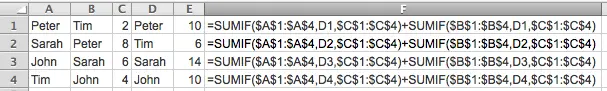
Pay careful attention to the use of absolute and relative references in the formula. I've created this formula in such a way that you can copy and paste the formula down from row 1 to row 4 without it breaking. However, if you wanted to add another row later, you'd need to edit the formula in the first row to include the new row ($A$5, $C$5, etc). Another option would be to name the range of cells and reference that name in the formula. Adding rows would then involve redefining the named range, which is a fairly simple process.
I've attached the spreadsheet I created for this example for you to download.
I hope this helps.
David
This is exactly what I was
This is exactly what I was looking for. Thank you.
You're welcome
Hi Bryan
Glad I could help!
Regards
David
If Statement between sheets
Hi,
I need an IF Statement that will compare the value of a cell in one sheet to a cell in another sheet, if they are the same, it needs to take the value of a different cell from sheet 2 and put it into the a cell in sheet 1. Any ideas?
Kelsey Layne
Need help in conditional formatting
if a1 is todays date and a6 is the due date i want a7 to come up with "paid" if paid on or before due date and "due" if passed due date
Comparing dates
Hi Vinesh
You don't say which cell contains the date when it was actually paid. For the sake of argument, I'll assume the following:
- A1 contains today's date
- A2 contains the date it was paid (blank if not yet paid)
- A6 contains the date it was due
If this sounds right, you could use a formula like this:
=IF(A2<=A6,"Paid on or before",IF(A1>=A6,"Due",IF(A1<A6,"Not yet due","")))
This formula does the following:
- Check to see if the bill was paid on or before the due date. Will return "Paid on or before" if it was, otherwise ...
- Check to see if todays date is after the due date, in which case return "Overdue", otherwise ...
- Check to see if today's date is before the due date, in which case return "Not yet due", otherwise ...
- Return "Due Today".
=if(AE14:AE14<=75,"B",if(AE14
=if(AE14:AE14<=75,"B",if(AE14<80,"D",if(AE14<85,"AP",if(AE14<90,"P", if(AE14<101,"A")))))
anyone who could help me on this formula..... thanks in advance....
More information please ...
Hi Lanie
Can you explain what the problem is?
I can see a couple of possible problems:
- Change AE14:AE14 to just AE14 in the first IF statement.
- You haven't VALUE_IF_FALSE value in the final IF statement. What happens if AE14 is not less than 101?
David
Hi David..
Hi David..
I am doing my class record, and i want the descriptive rating automatically displayed once the periodic rating are computed.
for example:
B2 C2
B2 cell is for periodic rating
C2 cell is for descriptive rating
here are the legend:
>74 below is B
>75-79 is D
>80-84 is AP
>85-89 is P
>90-100 is A
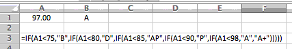
if the grade is 98, then on the descriptive rating must be displayed A...
Thanks for you help :) God bless..
Hi Lanie
Hi Lanie
Here's the formula I would use:
=IF(A1<75,"B",IF(A1<80,"D",IF(A1<85,"AP",IF(A1<90,"P",IF(A1<98,"A","A+")))))
The spreadsheet this comes from looks like this:
However, this is a scenario in which I'd use a VLOOKUP function rather than multiple IF statements in a single formula. It allows you to create a simpler formula, and you can change the gradebook more easily without having to change all of the individual gradebook formulas. You can read about the VLOOKUP function in this lesson.
Regards
David
hi thanks much for your help.
hi thanks much for your help... it works...
actually my first option is the vlookup function, but am having a problem in the pointing system, which is for example 89.90, i don't want to list all the decimal places for the vlookup, so i've come up to use the if statement formula.. :) :) :) many thanks to you.....
i still another questions if you don't mind? :D
More help?
Hi Lanie
Of course - happy to help. Fire away!
David
Multiple Conditions for IF Statement
I'm trying to do a formula that says if a cell is greater than one cell and less than another cell then I will have one message if true and another if false.
Using the AND function to evaluate multiple conditions
Hi Michele
You could do this in a couple of ways.
Let's assume you have the following cells:
- A1 contains the value you are comparing.
- A2 contains the value you want A1 to be greater than
- A3 contains the value you want A1 to be less than
The simplest option would be to use a single IF function combined with the AND function, like this:
=IF(AND(A1>A2,A1<A3),"Message if true","Message if false")
The AND function allows you to include two or more logical tests - in our case, these are "A1>A2" and "A1<A3". They are logical tests because each test will return either TRUE or FALSE. The AND function will also return TRUE or FALSE. For the AND function to return TRUE, all of the included logical tests must evaluate to TRUE. Therefore, this IF function will only return "Message if True" if both tests are true. The alternative to AND is OR, where only one of the statements would need to be true for the OR function to return TRUE.
Another option to solve your problem would be as follows:
=IF(A1>A2,IF(A1<A3,"Message if true","Message if false"),"Message if false")
This is clearly less efficient because we need to include the "Message if false" twice. In a very large spreadsheet you'd probably find that this solution slows the calculation speed of the spreadsheet. However, there are situations where it is more flexible than my first solution. However, I'd always start with the first solution because it's simpler!
I hope that helps.
David
Excel-2007
if i type in d5 or e5 then it will automatically perform this formula in f5 cell- "f4+d5-e5". but problem is if i input any one of d5 or e5 this have to perform that formula. please help.
Count with multiple conditions
Hello, I'm trying to find the formula for the count, with two if statements. I want the count of cells, if C2:C450 shows "N" and E2:E450 is "ACCORD". So for example, in order to be included in the count, C35 would have to show N, AND E35 would have to show ACCORD. Can you help me? I've tried so many different things and can't get it right!
Here's what I currently have, but it's obviously not giving me a value.
=COUNTIF(C2:C450,"N")*AND(E2:E450,"ACCORD")
need help to calculate time by category
Hi all genius...
i need help on how to create a formula to as below for running 2.4km based on the given time:
Age category A is 20~24, B is 25~29, C is 30~34, D is 35~39, & E is 40<above
For category A, Grade A is below 12min, B < 13min, C < 14min, & above 14mins id Failed.
pls help me ... thank u all...
solving discount of different percentages
hi
help with formula to generate discount for the items where laptop is given a discount of 12% tv = 9% and radio = 8%
the table is as follows:
item price discount
laptop 12000
radio 1000
laptop 45000
radio 15000
tv 50000
laptop 50000
radio 5000
laptop 65000
radio 2000
tv 21000
laptop 75000
Need help to calculate the Over Time amount based on day & OT hr
Hi,
Below is the sample date , I need help to calculate the OT based on day "Sunday" and based of "Total Duration". I has mentioned the sunday OT rate card also.
EmployeeName Date In Time Out Time Total Duration Ot Rate
abcd 01 Sep 2013 11:54:45 16:53:25 4:58:40
abcd 2-Sep-13 11:54:45 16:53:25 4:58:40
abcd 3-Sep-13 11:54:45 16:53:25 4:58:40
abcd 4-Sep-13 11:54:45 16:53:25 4:58:40
abcd 08 Sep 2013 10:24:52 16:03:51 5:38:59
Sunday OT Rate
<5=120
>5<8=230
>8=300
Calculating overtime with multiple IF functions
Hi Abraham
You can do this using a formula containing multiple IF functions like this:
=IF(E1<5,E1*120,IF(E1<8,E1*230,IF(E1>=8,E1*300)))
In this example, E1 contains the duration for the person you are calculating overtime for.
Note that my formula uses a slightly different table to yours. Your example would not have paid overtime for exactly 5 hours or exactly 8 hours. My formula will pay 230 for 5 hours and 300 for 8 hours. If you want to pay 120 for 5 hours and 230 for 8 hours, then use this formula instead:
=IF(E1<=5,E1*120,IF(E1<=8,E1*230,IF(E1>8,E1*300)))
I hope this helps.
Regards
David
Mutliple If/And with ranges
Hello. I'm trying to make a formula that will input the cost of a unit by two given variables.
This is what I was able to come up with so far:
Quantity Stitch Count Unit Cost
22 2000 ???
The scenario is that the person can input the quantity and stitch count of the item, and the unit cost will calculate the amount based on both arguments.
So I was able to come up with this formula to do that:
=IF(AND(AND(D3>=0,D3<=23),AND(E3>=0,E3<=5000)),D3*2.5,)
However I need to add a number more arguments in order to calculate any option the person could put in. When I try to add to the formula I receive an error for Value.
Stitches 1-23 24-35 36+
0 – 5000 $2.50 $2.00 $1.50
5000-6000 3.00 2.30 1.75
6000-7000 3.50 2.60 2.00
7000-8000 4.00 2.90 2.25
The stitches will go up to 16000, so I anticipate it to be a long formula.
Is this possible to accomplish? I hope this wasn't too confusing....
Nevermind
Nevermind! I was able to figure it out
Need "If" formula
Hi,
I have date & time as 10/14/2013 12:24:00 PM in cell A2 and in cell A3 I have data & time as 10/15/2013 00:15:00 AM, I need a "IF" formula in cell A4 which gives me "Ontime" if the cell A3 date and time is within 10/14/2013 23:59:00 and If date and time is greater than 10/15/2013 00:01:00 AM it should give me as "Delay in report"
Help Needed: If/Then, Multiple Conditions
In my scenario we have three Material Markups: A and B are specific to Items L and R, and C which applies to all other items
We also have three Item Types: L and R are specific and S is a standard which not L or R
Here is the logic:
If ITEM = A, then Markup L, FALSE use Markup S
If ITEM = B, then Markup R, FALSE use Markup S
If ITEM <> A or B, then Markup S.
The formula I came up with will not address all the variables. Any help would be appreciated! Thank you.
Use a formula with nested IF statements
Hi D
You need to use a formula like this:
=IF(item=A,markup L,IF(item=B,markup R,markup S))
- The first IF function evaluate the item to see if it is A.
- If it is, then Markup L is applied.
- If it is not, the next IF function determines if the item is B.
- If it is, then markup R will be applied.
- If it is not B, Markup S will be applied.
Because the IF functions are nested in this way, S will be applied if the item is neither A nor B. The only time the second IF function will be used is if the item is not A, which means that if the second IF function finds that the item is not B, then we already know it is not A, so Markup S must therefore be applied.
This is obviously a simple example. You could have a scenario where you have items of type A,B,C,D,E,F with markups to match. In a more complex scenario such as this, I'd consider using the VLOOKUP function instead of a formula with nested IF statements as we have here. You can read our VLOOKUP lesson here.
Regards
David
multiple 'ifs'
Hi, I am trying to get the results of a test to include an average of various parts of the test, that means that the numerical result will not necessarily be a whole number. Then I want convert the number in to a grade, A1, A1+1 etc. For some reason the formulae I have created don't work; can you see why? I've been over it several times and have reached a dead end!
=IF(B13<1,"-A1",IF(B13=1,"-A1",IF(B13<=1.5,"-A1",IF(B13>1.5,"A1",IF(B13=2,"A1",IF(B13<=2.5,"A1",IF(B13>2.5,"A1+1",IF(B13=3,"A1+1",IF(B13<=3.5,"A1+1",IF(B13>3.5,"A1+2",IF(B13=4,"A1+2",IF(B13<=4.5,"A1+2",IF(B13>4.5,"B1",IF(B13=5,"B1",IF(B13<=5.5,"B1",IF(B13>5.5,"B1+1",IF(B13=6,"B1+1",IF(B13<=6.5,"B1+1",IF(B13>6.5,"B1+2",IF(B13=7,"B1+2",IF(B13<=7.5,"B1+2",IF(B13>7.5,"C1",IF(B13=8,"C1",IF(B13<=8.5,"C1",IF(B13>8.5,"C1+1",IF(B13=9,"C1+1",IF(B13<=9.5,"C1+1",IF(B13>9.5,"C1+2",IF(B13=10,"C1+2",IF(B13<=10.5,"C1+2",IF(B13>10.5,"C2",IF(B13=11,"C2",IF(B13<=11.5,"C2",IF(B13>11.5,"C2+"))))))))))))))))))))))))))))))))))
thanks for any advice!
Multiple ifs
I have to solve a formula which divides the gross between 2 companies with min comp. If its <$24/day co1 gets 100% if >$24<$48 Co2 gets 100%
>$48 goes 50% to both companies. Can I use IF formula for this?
# of Days "Gross
Collected"
36 578.60
24 449.75
32 642.00
42 680.50
31 581.75
25 562.75
24 563.75
42 1,056.25
21 554.25
42 1,045.00
18 595.00
thanks
Yes, the IF function will do this for you
Hi Egs
The IF function will work for you here but you'll need two formulas - one to calculate company 1's share of the gross and one to calculate company 2's share of the gross.
You have described three possible outcomes, which means we need two IF functions in each formula.
Lets assume that the # Days is in cell A1, and the Gross is in B1. We'll calculate company 1's share in C1 and company 2's share in D1.
In C1, enter this formula:
=IF(A1<24,B1,IF(A1>=48,B1*50%)
In D1, enter this formula:
=IF(A1<24,0,IF(A1<48,B1,B1*50%)
This should solve the problem you've described.
Regards
David
coming up with False
Hi Dave,
I am trying to make this work but no success. It's coming up with False value. I have min comp for 2 companies.
Co1 gets (31days*$24) at any values. Sp if the values is < 24 co1 gets it all. then if value is >$24/day Co2 gets >24*31 up to (48*31days) 100% then whatever is over both min comps goes 50% to both co.
thanks a bunch
Your logical tests are the problem
Hi Steve
In this case, the fourth IF function is the problem. The logical test in that function is B13>1.5. If this test is TRUE, the IF function will return A1, and Excel will ignore everything that comes after it. The way you've set it up, this test will always be true. Reading through the formula, it looks to me like the logical test in in this case should be B13<2. This will catch all values greater than 1.5 and less than 2.
In addition, you've repeated this error multiple times by having multiple IF functions that use a greater than test rather than a less than test. You'll need to fix each of those in the same way.
Two further points:
- Our VLOOKUP lesson will show you a method of returning grades that is WAY easier than using multiple IF functions.
- If you want to stick with multiple IF functions, you can write this function in a much simpler way.
To simplify this function, look at the first portion of your formula:
=IF(B13<1,"-A1",IF(B13=1,"-A1",IF(B13<=1.5,"-A1"
In this case, you've tested B13 for three separate values, yet the TRUE value has been "-A1" every time. Why not just write this:
=IF(B13<=1.5,"-A1"
If you decide later to have different grades for different values below 1.5, then add back more IF functions. But for now, you've got two IF functions that you dont' need and which are simply complicating your formula. And if that scenario is a possibility, then a VLOOKUP function will make like a lot easier for you.
Hopefully that helps.
Regards
David
David, many thanks for your
David, many thanks for your excellent advice! I am changing the whole thing to use vlookup as you suggest and it already works as it should! Thanks for taking the time, much appreciated.
Need Help with Nested IF Function based on multiple criteria
I need an IF Function to calculate the Rating column based on two percentages. (the EOY Group Results with the EOY Achieved result). Any assistance would be great. Example of what I need calculated is listed below.
Performance Element EOY Group Results EOY Achieved Results Rating
New Hire Retention Rate 82.9% 76.5%
Criteria is as follows:
If the Achieved Result is
1- 5 or less percentage points below the EOY Group Result (the rating result should return a 4)
2- Less than 8 but more than 5 percentage points below the EOY Group Result the rating result should return a 3)
3- Less than 10 but more than 8 percentage points below the EOY Group Result (the rating result should return a 2)
4- More than 10 percentage points below EOY Group Result (the rating result should return a 1)
Here is what I have so far but it doesn't seem to be working for me. Based on my calculations for the about two percentages I should be getting a rating result of 3 but each time I play with the formulas I come up with a 4 or a 1
Any help would be greatly appreciated.
=IF(C7<B7-10%,1,IF(C7<B7+10%>B7+8%,2,IF(C7+5%<B7-8%,3,IF(C7<B7-5%,4))))
You need to nest the IF statements in the right order
Hi Paul
The problem with your formula is the way you've structured it. Specifically, your logical test in the second and third IF statements. Excel can't evaluate a logical test like "C7<B7+10%>B7+8%", so it will return FALSE every time. So your formula is currently returning 1 if C7<B7-10%, or 4 in all other cases. There is a way for the IF function to handle complex logical tests like the ones you've used, by using the AND or OR logical functions, which you can read about here. However, I think you can handle your requirements with just nested IF statements. Keep reading to find out how.
Looking at your criteria for assigning ratings, the first test is fine.
The second test should be C7<B7-8%. This test will only be required if the first test returned false. In other words, the only time this test is needed is if C7 is NOT less than B7-10%.
Similarly, the third test should be C7<B7-5%. The first two IF statements already established that C7 is not less than B7-10%, and C7 is not less than B7-8%.
Finally, it looks to me like the fourth test should actually be C7<B7. If the formula gets as far as evaluating this test, then we know that the value in B7 must be greater than or equal to B7-5%. However, I assume that this formula should return anything if C7=B7 or C7>B7. Therefore, C7<B7 is the right test.
With all that in mind, here's what the final formula should look like:
=IF(C7<B7-10%,1,IF(C7<B7-8%,2,IF(C7<B7-5%,3,IF(C7<B7,4,""))))
Note that I've added a value_if_true to the final IF statement. This will ensure that nothing is returned if C7>=B7. If you leave the final value empty (which is OK when using the IF function) then the formula would return FALSE in this scenario.
I hope this solves your problem - let me know if it doesn't. Also, you might find the VLOOKUP function helpful as an alternative to using nest IF statements. You can view our VLOOKUP lesson here.
Regards
David
Calculations using percentages instead of $ figures
Hi there. I do understand how this example is functioning, but I'm trying to use it with a group of percentages....and it's not functioning. What am I missing? Example: If the margin% cell is 0-49% then calculate the total sale cell by 0%. If the margin cell is 50-54.99%, then calculate the total sale cell by 3%. Am I barking up the wrong tree?
Hi Marie
Hi Marie
Based on what you've described, I'd write the IF function like as follows:
Let's assume that the Margin% cell is A1 and the Sales cell is A2:
=IF(A1<50%,0,A2*3%)
This formula looks at the Margin% cell in A1 and checks if it is less than 50%. If it is, then the IF function returns zero. If not, then it returns the result from multiplying the Sales cell by 3%. In this case it would return 3% of the sales value. If you wanted to return the sales value plus 3% instead, then use A2*103%.
Note that you only need one IF function in this scenario, because there are only two possible outcomes (0-49% or 50%-54.99%)
If you had a third possible outcome, 55%-60%, with a percentate of 3.5%, then the IF function would look like this:
=IF(A1<50%,0,IF(A1<55%,A2*3%,A2*3.5%))
You could keep on extending it in the same way for additional outcomes. However, once you get past 3-4 IF functions in the formula, I'd suggest you consider using a VLOOKUP function instead, where you look up the margin amount in a table which returns the correct percentage to multiply the sales amount by. This has three advantages over multiple nested IF functions:
- The formula is a lot less complex.
- You can change the percentages in the table and all of the formulas automatically recalculate (i.e. you don't have to edit the formula to reflect the new percentages)
- You can make the table larger (more rows) without having to add extra IF statements to handle the additional outcomes.
You can view our VLOOKUP lesson here.
Hopefully this helps. Let me know if I've missed anything.
David
David, Thanks so much, I'm
David, Thanks so much, I'm pleased to report that at the 11th hour, I figured it out on my own. Here's what I came up with:
IF(AND(I22<=49.99),D22*0%,IF(AND(I22>=50,I28<=54.99),D22*3%,IF(AND(I22>=55,I28<=59.99),D22*4%,IF(AND(I22>=60),D22*5%,"Out of range")))) Works like a charm. One of the biggest issues was the simplest fix, my column was formatted to text instead of number. *facepalm*
MG
Can Some one help me solve this problem?
I duno how to write this formula.
Here got 48,59,68,79,98and 109.
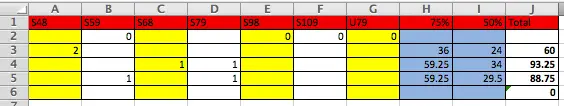
on the table show 98 have 2,68 have 3 and 59 have 1. I wan take the heighest 98x75% and other is 50%.
98 X 75% = 73.5
(59+(68X3)+98) X 50%=180.5
Thanks For helping me solve this problem
Can you confirm some details?
Hi Xavier
Thanks for your question. I've looked at the spreadsheet you uploaded and I can't figure out what you're trying to do. I've included a screenshot here - can you explain again what you want to achieve?
Regards
David
Sales drop formula
to find sales drop, eg. jan qty100,feb70,mar-55,april-48 ( if feb sales qty <30% march sales qty <20%, and april sales qty <10%, then there is sales drop) pls. help me for formul
Use the AND function
Hi Saji
You can use multiple IF functions in a formula to achieve ths, but you can also use one IF function and combine it with the AND function.
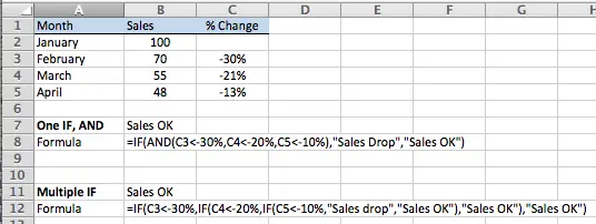
As you'll see from the screenshot, the first example uses just one IF function, combined with the AND function for the logical test. This formula is much shorter and easier to troubleshoot than the second example which uses multiple IF functions, and which needs to repeat "Sales OK" for each IF function we use. We could write the second formula without using "Sales OK" three times (i.e. the value_if_false argument of the IF function), but then our formula would return "FALSE" in some cases.
The AND function works by taking two or more logical statements and evaluating whether each is true. If they are all true then the AND function returns TRUE. If any of them are false then the AND function will return FALSE. You can read more about the AND function and its partner, the OR function, in our lesson on logical operators in Excel.
I hope this helps.
Regards
David
Thanks for reply,
Thanks for reply,
Im not familier in excel formula, actually i need formula for below data, pls. help me out.....
jan feb mar april remark
100 60 40 30 sales drop
100 90 100 60 sales ok
100 100 100 100 sales ok
or
jan feb mar april sales drop
100 60 40 30
"if feb sales less than 30% of jan sales, and if mar sales < 20% of feb sales,
and if april sales <10% of mar sales ""sales drop"",sales ok"""
Help with formula
What I need to be able to do is when a vehicle number is input in the top part of the sheet, rows 3-29, rows 31-40 need to highlighted for the corresponding day the vehicle will be out. The info at the top part of the sheet is variable, the bottom part is static.
I need to return a Particular letter based on a series of cells
I have a worksheet where I need to determine if someone is a new, current, or reactivated customer. The cells are based on total earnings for a year (example:)
C7 = $1200
D7 = $1300
E7 = $800
F7 = $1200
Then L7 should return an "C" for current customer. However, if all cells but F7 are 0, then L7 should return an "N" for new customer, and if E7 (or D7 and E7) are zero and both C7 and F7 have a number, then an "R" for reactivated customer.
I have clue how to create this formula, or if it is even possible. I hope I made sense.
Can you confirm some details?
Hi Glenn
Thanks for your question. The answer should actually be pretty simple, but when I looked at the spreadsheet you uploaded it didn't quite match the scenario you described:
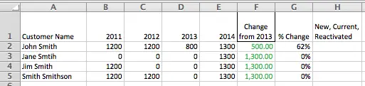
As you'll see, the numbers and cell references you described in your question aren't exactly as shown above. Can you confirm how you want your solution to work and I'll see what I can do.
Regards
David
Clarification
Thanks, David! I replied to your comment, I am not sure if you will see it...so I am trying again.
I have uploaded the spreadsheet I am using, the example that I uploaded at first was just a dummy, none of the columns were correct. the new spreadsheet, you will see that the columns are as they were in my example, however the row numbers are not. I included four different customers with each of the scenarios I suggested in my original question.
I hope this helps!
Thanks, Glenn!
Clarification
Thank you for your response, as well as the opportunity to learn a new skill!!
In the example spreadsheet I uploaded I put in four "customers" where I would enter their purchases for a year. What I am seeking to do is have a formula that would simply return a value of "N", "C" or "R" once all the sales years are input.
There were some columns that I didn't think were necessary to the formula, but I can understand the confusion.
I have uploaded the same example on the spreadsheet that I am using. The only difference is instead of it beginning on C7, it begins on C2.
Thank you again!
Glenn
Thanks!
Glenn
help in a formula
i, I desperately need help writing this IF Statment. I could not figure it out to save my life
a. 2011 Income Taxes: (This requires an If Statement.) If 2011 Income Before Taxes is less than zero, then 2011 Income Taxes = 0; otherwise 2011 Income Taxes = 40% * 2011 Income Before Taxes. (If you CANNOT figure this out, type in the correct numbers manually; I will know by your formulas worksheet.) The manual numbers are: 1,326,036; 0; 550,874; 0; 927,156
Revenue $ 131,201,647
Cost of Goods Sold $ (17,213,872,044,311,000)
Gross Margin $ 17,213,872,175,512,600
Expenses
Advertising $ 19,680,347
Rent $ 1,800,000
Salaries $ 23,616,296
Supplies $ 1,968,025
Maintenance $ 2,100,000
Total Expenses $ 49,164,668
Income Before Taxes $ 82,036,979
Income Taxes $ 1,326,036
Net Income $ 80,710,943
I am not sure that I set up the cost of goods sold correctly. The amounts seem very high. I used
=B4*(1-$B$4) as my formula.
I appreciate any help that you can give me.
IF function
I have a bonus structure based on revenue over $20,000. For every $1000 over $20,000, $50 is added to pay.
example 21000 would equal an extra 50, but then next 50 wouldn't come until it hit 22,000. Still just 50 if revenue hits 21,800 for example.
Simple formula to calculate commission
Hi Tyler
There are a number of ways to solve your problem. If it is always as simple as this, I'd do it like this:
=IF(A1>20000,ROUNDDOWN((A1-20000)/1000,0)*50,0)
This will do the following:
- Check if the value in A1 is greater than 20
- If it is, then do this:
- Take the sales amount and subtract your base revenue ($20,000)
- Divide that by $1000
- Round the result down to zero decimal places.
- Multiply that by $50.
- If it isn't, then return 0.
You could also use the following formula to get the same result without using the IF function:
=(ROUNDDOWN((A1-20000)/1000,0)*50)*(A1>20000)
This uses the same function as above to calculate the commission amount, and then multiplies it by the result obtained by comparing A1 to 20000.
- If A1 is less than 20000, then the result of (A1>20000) is FALSE, or zero. Multiplying this by the results of the commission amount will result in the whole formula returning 0, which takes care of the scenario where the ROUNDOWN function will return a negative commission amount for sales values less than 20000.
- If A1 is greater than 20000, then the result of (A1>20000) is TRUE, or 1. The formula will then return the correct commission.
The second example uses Excel's Logical Operators to avoid using the IF function. You can read more about logical operators in Excel in our lesson here.
Regards
David
Need help to create formula
Hi need help with formula (True or False argument) for Column L.
If any cell in the rows in the table match the numbers from Supp cells (H23, I23), return a TRUE value in column L
DO NOT match.................................................................return a FALSE value
Use the OR function to solve your problem
Hi Bob
Your problem is a lot simpler than you'd think. To summarise what you're doing:
- You have several rows of numbers
- You need to check whether the values in two "Supplementary" cells are found anywhere in each of those rows of numbers.
- If they are, then your formula should return TRUE, otherwise they should return FALSE.
Here's a screenshot of your spreadsheet:
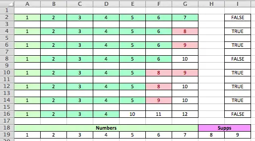
The formula I would use here looks like this:
=OR(COUNTIF(A2:G2,$H$19)>0,COUNTIF(A2:G2,$I$19))
This is the formula for I2 in the example above, but you could copy and paste it into the other cells in column I.
The formula works like this:
- The OR function is a logical function in which you enter two or more logical tests.
- If either test is true, then OR returns TRUE as well, otherwise it returns FALSE.
- I've used just two logical tests in your example:
- Use the COUNTIF function to count the number of instances of the value in H19 (which is 8), and then check if the result is greater than 0. In the first row of numbers, 8 doesn't occur so the COUNTIF function returns 0, so this logical test returns FALSE because 0 is not greater than 0.
- Similarly, use the COUNTIF function to count the number of instances of the value in I19 (which is 9), and then check if the result is greater than 0. In the first row of numbers, 9 doesn't occur so once again the COUNTIF function returns 0 and the logical test returns FALSE.
- In the first row, since neither 8 nor 9 appear in the row, the result of the formula is FALSE. As you can see in the screenshot above, those rows that contain either 8 or 9 return TRUE, as required.
Note that if you only wanted to return TRUE if both 8 and 9 appeared in the row, you would use AND instead of OR in the formula (nothing else would need to change).
You can read our lesson about the COUNTIF function here.
You can read more about the AND and OR functions in our lesson on logical operators and functions here.
Both links open in a new window.
Let me know if that solves your problem, or if there's anything else you need.
Regards
David
Thanks for that, it works
Thanks for that, it works great! I didn't think of the OR function, when I was trying the IF function I could get it to work on just 1 cell in the table to 1 cell from the the SUPPS, but not multiple cells. also I am self teaching myself how to apply logical functions in exel.
thanks again.
Bob
Hi David,
Hi David,
I have another problem is when I copied the sheet (OZ-Lotto) and named new sheet (Lotto), the formulaes in Column H (Division Win) wont work, is there a problem simply coping some formulaes from 1 sheet to another?
spreadsheet in excel use IF function
I have 3 requirement for employees which will give annual bonus @2% of their base salary.
The requirement are take medical certificate not more than 6 days,annual leave only 7 days and absence without notice can not more than 1.
If all the requirement can be fill by the employee then the employee will get @2% of his salary.
But when I compute into excel,excel not really can give accordingly what I want.
what formula should I use for this category?
Thanks
I would use the AND function here
Hi Ceri
I would use the AND function. The AND function looks at 2 or more logical tests and returns TRUE if all of the tests are true, and FALSE if one or more of the tests are false.
Here's an example based on the information you supplied:
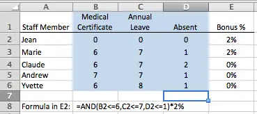
The function uses a logical test for each of your three criteria:
- B2<=6 (Medical certificate no more than 6 days)
- C2<=7 (Annual leave no more than 7 days)
- D2<=1 (Absent no more than 1 day)
The AND function evaluates these tests for each person and returns TRUE or FALSE for each. If all three tests are TRUE, as they are for Jean and Marie, then the AND function returns TRUE as well.
The formula then multiples the result of the AND function (TRUE or FALSE) by 2%. Because TRUE is stored as 1 by Excel, and FALSE is stored as 0, the formula will return a bonus of 2% if TRUE or 0% if FALSE.
I hope this helps. You can read more about using the AND function and its partner function OR in our lesson on logical operators. This link will open in a new tab.
Regards
David
If function
Great Lesso!! helped me to understand If function and create my If formula I needed. Thank you
make formula with if with multiple variables in each column
Dear Sir,
I have made some formulas with "if ".Now I want to accommodate the variables of various columns as indicated in table. For exam if I want to calculate the Dia of conductor then first I select w.o.,then material (copper or alluminium),then type of conductor(S- solid,F- flexible like wise).In similar ways in Insulation & other req. field I want to accommodate the possible variables in my formula.
Can you help me?
Best Regards & thanks in anticipation,
Ashijeet
I needed an quick answer
I needed an quick answer about multiple IF statements and your post was near the top of the list, VERY easy to follow, and I had my formula done in less than 5 minutes. Thanks for posting this. You helped me greatly.
Excel Help
Can this be done, I think only nested loop can work, but question want something else. Please reply fast.
Tickets for Pilots basketball games can be purchased according to the following schedule:
Price/ticket for first 10 tickets $10
Price/ticket for next 10 tickets (11-20) $8
Price/ticket for tickets > 20 $6
Compute ticket prices for following tickets bought by three individuals by using only one IF function
8
16
39
Error Message
I re-created the same table used in your example, and I understand all the different steps and the logic behind it. However, when I want to re-create the same formula (I even copied and pasted your formula), I always get error messages that something is wrong in the formula. I checked it many times and it is exactly like the formula in the example. I am not sure what I do wrong. Can you help me with this?
Can you upload your spreadsheet?
Hi Tanja
Could you upload your spreadsheet in a reply to this comment and I'll take a look at what might be wrong.
Regards
David
Here is the file!!!
Thank you, David. Here is the file. I am using Excel 2007.
Sorry here it is!
Sorry here it is!
Again!!! Sorry about that!
Again!!! Sorry about that!
I see the problem ...
Hi Tanja
I can see the problem - you're using semi-colons instead of commas in the formula.
Regards
David
formula
Hello,
I work for a bank and im trying to create a formula to calculate which rate a loan will be offered.
We have 3 loan types 1, 2 or 3
Each loan type will have a score. <9, between 9-12, 13-16, 17-20. Their rate will depend on what type they are and what score they have.
I've attached a spreadsheet that shows the types, score and which rate will be offered.
Any help would be greatly appreciated.
Thank you
Pamela
Got it on my own!
Got it on my own!
=IF(AND(F2=1,G2>16),6,IF(AND(F2=1,G2>12),7,IF(AND(F2=1,G2>8),8,IF(AND(F2=2,G2>16),5.5,IF(AND(F2=2,G2>12),6,IF(AND(F2=2,G2>8),6.5,IF(AND(F2=3,G2>16),4.75,IF(AND(F2=3,G2>12),5,IF(AND(F2=3,G2>8),5.5,0)))))))))
Bonus tracker help
Hi there,
I'm stuck on the formula...getting several error messages.
Trying to have the column titled "productivity multiplier" come up with a % based on the previous column "Performance Percentage".
If performance percentage is:
0-79%, then multiplier column should input 0%
80-89%, then 10%
90-99%, then 15%
100-109%, then 20%
110-119%, then 25%
120-129%, then 30%
130-139%, then 35%
140-149% then 40%
150-159% then 45%
160-169% then 50%
above 170%, then 55%
I tried this formula: IF(D2<80%,"0%",IF(D2<90%,"10%",IF(D2<100%,"15%",IF(D2<110%,"20%"....etc
I also tried eliminating that the multiplier column and using this formula in the TOTAL BONUS column: =IF(D2<.80,E2*0%,IF(D2<.90,E2*10%,D2<1.00,E2*15%,IF(D2<1.10,E2*20%,IF(D2<1.20,E2*25%,IF(D2<1.30,E2*30%,IF(D2<1.40,E2*35%,IF(D2<1.50,E2*40%,IF(D2<1.60,E2*45%,IF(D2<1.70,E2*50%,E2*55%)))))))))
I also tried percents rather than decimals based on some of your other instructions but I am getting an error that there are too many statements.
If you see what I am doing wrong or how I can resolve this, it would be MUCH appreciated!
For long nestings
So I have a 100 items that I need nested as if statements like this, but when I put it into excel it says the limit of nested statements is 64. Is there some way to get around this or use a different method?
Nested IF statment
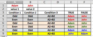 Please help me how to use if statement with attached table
Hi Ali
Hi Ali
It looks to me like this problem can't be solved. Here's why:
- In row 4, you have ODD, ODD, A2<B2.
- The table says that if A2<B2 then the outcome is Adam, otherwise it is John.
- In row8, you have ODD, ODD, A2=B2.
- The table says that if A2=B2 then the outcome is Adam, otherwise it is John.
- The outcomes of row 4 and 8 contradict each other:
- The test in row 4 says that if A2 is not less than B2, the outcome must be John.
- The test in row 8 says that if A2 equals B2 then the outcome must be Adam.
- However, if A2 is not less than B2, then it could be equal to B2. Which one should we choose - John or Adam?
It looks like you need to restate your table to reflect a set of mutually exclusive outcomes.
Regards
David
Alternatives to multiple nested IF statements
Hi Katya
Thanks for your email. I've pasted your formula here so other readers know what we're talking about. It's not the first time I've come across an overly complicated formula based multiple IF function like, so I figure it's worth sharing this simple solution with everyone!
=IF(F2<25,1,IF(F2<25,2,IF(F2<50,3,IF(F2<100,4,IF(F2<150,5,IF(F2<200,6,IF(F2<400,7,IF(F2<600,8,IF(F2<800,9,IF(F2<1000,10,IF(F2<1500,11,IF(F2<2000,12,IF(F2<3000,13,IF(F2<4000,14,IF(F2<5000,15,IF(F2<6000,16,IF(F2<7000,17,IF(F2<8000,18,IF(F2<9000,19,IF(F2<10000,20,IF(F2<11500,21,IF(F2<13000,22,IF(F2<14500,23,IF(F2<16000,24,IF(F2<17500,25,IF(F2<19000,26,IF(F2<20500,27,IF(F2<22000,28,IF(F2<23500,29,IF(F2<25000,30,IF(F2<27500,31,IF(F2<30000,32,IF(F2<32500,33,IF(F2<35000,34,IF(F2<37500,35,IF(F2<40000,36,IF(F2<42500,37,IF(F2<45500,38,IF(F2<47500,39,IF(F2<50000,40,IF(F2<55000,41,IF(F2<60000,42,IF(F2<65000,43,IF(F2<70000,44,IF(F2<75000,45,IF(F2<80000,46,IF(F2<85000,47,IF(F2<90000,48,IF(F2<95000,49,IF(F2<100000,50,IF(F2<110000,51,IF(F2<120000,52,IF(F2<130000,53,IF(F2<140000,54,IF(F2<150000,55,IF(F2<160000,56,IF(F2<170000,57,IF(F2<180000,58,IF(F2<190000,59,IF(F2<200000,60,IF(F2<210000,61,IF(F2<220000,62,IF(F2<230000,63,IF(F2<240000,64,IF(F2<250000,65,IF(F2<260000,66,IF(F2<270000,67,IF(F2<280000,68,IF(F2<290000,69,IF(F2<30000,70,IF(F2<310000,71,IF(F2<320000,72,IF(F2<330000,73,IF(F2<340000,74,IF(F2<350000,75,IF(F2<360000,76,IF(F2<370000,77,IF(F2<380000,78,IF(F2<390000,79,IF(F2<400000,80,IF(F2<410000,81,IF(F2<420000,82,IF(F2<430000,83,IF(F2<440000,84,IF(F2<450000,85,IF(F2<460000,86,IF(F2<470000,87,IF(F2<480000,88,IF(F2<490000,89,IF(F2<500000,90,IF(F2<510000,91,IF(F2<520000,92,IF(F2<530000,93,IF(F2<540000,94,IF(F2<550000,95,IF(F2<560000,96,IF(F2<570000,97,IF(F2<580000,98,IF(F2<590000,99,IF(F2<600000,99,100)))
I would use a VLOOKUP function to solve this specific problem. There are other ways you could do it, but this is the simplest and easy to manage once you've set up the initial table.
- With this, you can look up a value in a table of data and then retrieve the appropriate value that relates to the item that matches your lookup value.
- The table of data in your case would look something like this (I've only done part of it but you could easily extend it to cover all of your potential values):
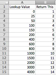
- Your formula would then look like this (assuming the value you are looking up is in F2):
=VLOOKUP(F2,$A$2:$B$14,2,0) - This formula looks down the first column in the table for a match with the value in F2.
- If it can't find one, it stops when it finds a value that is larger than the value in B2, then drops back one row in the table.
- It then selects the value from column 2 in the table, which is the result of the formula.
- Note that it is very important that the table is sorted by the values in the first column starting with the smallest value.
- Also, if it is possible for the lowest value of F2 to be less than 0, then you should put the lowest possible value in A2 in the example shown.
I suggest you read our lesson on VLOOKUP functions to find out more about how the VLOOKUP function works. Let me know if you still have any questions.
Regards
David
Help Please ~
If someone could please help me write an IF statement for the below problem:
The evaluation must total points based on an "X" being in the box.
Ex: if the user checks "X" total the associated points in a box below. I have only gotten as far as: =IF(N114="x", sum)
YES: 50 NO: 0
YES: 25 NO: 0
Thank you!
Please Help
Hello,
Does anyone can help me to solve this problem.. i want to know how to write the formula for my example.
Status is refers to the last cell that filled in one row.
Please help me.
Regards,
Yanson.
Please Help
Hello,
Does anyone can help me to solve this problem.. i want to know how to write the formula for my example.
Status is refers to the last cell that filled in one row.
Please help me.
Regards,
Yanson.
BIG Help
Just wanted to say thanks for this topic. I was trying to modify my time card calculations from =IF(AND(C12<>"",D12<>""),TEXT(D12-C12,"HH:MM")*24,"") to something that would include if went into next day and knew I just needed it to add 24 if the number wasn't greater than 0. Thanks to the beginning of this topic I was able to get to =IF(AND(C12<>"",D12<>""),IF(D12-C12>0,TEXT(D12-C12,"HH:MM")*24,TEXT(D12-C12+24,"HH:MM")*24),"") and solve my issue. I had to figure out to move the last "" to in between the two parenthesis but with a lie or two from excel I got it right. Thanks again.
multiple IF statement
Thank you very much. this was very useful to me.
Including an option for ERROR
Hi,
Thanks so much for all the help you have provided everyone, I've learned so much just reading through the page.
I'd like to set up my stacked IF statements to have the option that if nothing is listed, instead of returning an ERROR (or #N/A) it returns a value of $0. Here is the statement I have, that works if something is input to J8, but as I said, if J8 is blank, I'd like the result of the formula to be $0.
=IF($J$5="Perotti",VLOOKUP(J8,perotti,2,FALSE),IF($J$5="aidan",VLOOKUP(J8,aidan,2,FALSE),IF($J$5="bbag",VLOOKUP(J8,bbag,2,FALSE),IF($J$5="kyle",VLOOKUP(J8,kyle,2,FALSE),IF($J$5="fantl",VLOOKUP(J8,fantl,2,FALSE),IF($J$5="jim",VLOOKUP(J8,jim,2,FALSE),IF($J$5="cernig",VLOOKUP(J8,cernig,2,FALSE),IF($J$5="aj",VLOOKUP(J8,aj,2,FALSE),IF($J$5="dookoo",VLOOKUP(J8,dookoo,2,FALSE),IF($J$5="casey",VLOOKUP(J8,casey,2,FALSE),IF($J$5="eric",VLOOKUP(J8,eric,2,FALSE),IF($J$5="liam",VLOOKUP(J8,liam,2,FALSE)))))))))))))
Thanks so much!
Commission Calculation
Thanks for such a useful forum. I am struggling with a complex (for me ) commission structure and wondering if you can assist. I have 5 sales people who have their sales commissions calculated based on gross profit (GP). I’ve attached a spreadsheet with the escalating commission structure. If the GP is 29% or less they get commission of 2% of their total sales, if their GP is 30% to 31%, they receive 5% of the total sales, etc. I’m trying to create a running worksheet that will allow me to calculate each salespersons commission on a monthly basis with a running total in following months. I am having trouble with the formula. Would you be so kind as to assist? Thanks in advance for your assistance and the wonderful education you provide us with.
Best,
--Doug
Excel Vlookup Problem
Hi,i have 3 columns (Ticket Number , Site ID and Time) , i need to copy Site ID and Down Time according to the Ticket Number from 1st Excel sheet to 2nd excel sheet
For Example : I Have Ticket Number 425665 with Three Site ID's UW_GJ_2904 , UW_GJ_1995 , UW_GJ_0960 , So i need to copy all three site id's from 1st Excel sheet to 2nd excel sheet .... But as per vlookup only first site ID is Reflecting UW_GJ_2904 is Reflecting in all three places, which it should not(in some cases for single ticket Ex: 425771 : only one site UW_GJ_0514 will be there, it was reflecting properly, The problem is for each ticket which has more than one site ID is not reflecting properly)
First Excel Sheet :
Ticket Site id Down time
425665 UW_GJ_2904 1/21/14 4:51 PM
425665 UW_GJ_1995 1/21/14 4:51 PM
425665 UW_GJ_0960 1/21/14 4:51 PM
Second Excel Sheet:
ticket site id down time
425665 UW_GJ_2904 1/21/14 4:51 PM
425665 UW_GJ_2904 1/21/14 4:51 PM
425665 UW_GJ_2904 1/21/14 4:51 PM
if it is only one id its Reflecting properly
First excel sheet:
425771 UW_GJ_0514 1/21/14 7:44 PM
Second Excel Sheet:
425771 UW_GJ_0514 1/21/14 7:44 PM
IF Functions w/ Text
Hi,
Just wondering if any of you could help with how to write an IF function with multiple arguments but with text? Thanks in advance.
Here's the Context: we've got a product that lowers fuel consumption, though its effectiveness varies somewhat by industry.
Here's What I Want to Do: create a 3-stage simplified savings calculator. First, from a drop-down list users would specify what industry they are in (which will determine the fuel consumption decrease). Second, users would type in their annual fuel costs. Then they'll hit a button saying 'Calculate'. Their fuel costs will then be multiplied the fuel consumption decrease that is derived from the chosen industry.
Thus, if they choose 'Transport' as their industry (which relates to fuel savings of 8%), and put in $1,000,000 as their annual fuel costs, they will get a figure of $80,000 for their potential savings ($1m*0.08).
I've been able to do this on a sector-by-sector basis but haven't been able to combine them into a 'one-stop-shop' IF function.
The formula I've been using is =IF(B1="Transport", "0.08","0.00"), =IF(B1="Shipping", "0.1","0.00"), =IF(B1="Fishing", "0.12","0.00"), etc.
Any and all help is very much appreciated.
Thanks
Try a VLOOKUP function instead
Hi John
I'd suggest you look at our lesson on VLOOKUP. Based on the information you've given me, you need a reference table of data with the Industry in the first column, and the savings relating to that industry in the next columns.
Then, when someone chooses an industry, the VLOOKUP function will look in the reference table for a matching value and can then retrieve the savings from the second column. You can then multiply that by their annual fuel costs.
The VLOOKUP formula will look something like this:
=VLOOKUP(B1,Reference_table,2,0)
This says:
- Look for the value in B1 in the table Reference (you can name your reference table or simply refer to it using cell references, e.g. D1:E50.
- When you find a value, retrieve the data in the second column on that row.
Note that the 0 at the end of the formula tells VLOOKUP to look for an exact match in the first column of the table.
You can read more about the VLOOKUP function and how to use it here.
Regards
David
Great! Thank you.
This was very helpful. I used the multiple ifs in a score sheet for swimming meets. If 1st place then 6 points, if 2nd place 4 points, etc. Very useful and easy to use. Thanks for the post!
IF condition
Kindly help me put IF condition formula for below requirement,
Student Test marks % of attendance Test marks % of attendance Result Attendance
Sub 1 sub 1 sub 2 sub 2 Class
1. Paul 25 75% 35 85% First Shortage.
2. Max 35 85% 35 100% Distinction No
3. Harry 24 100% 25 100% Fail No.
Please consider following points.
Test grades equal to 25 - pass.
less than 25- fail
between 25-34.99 - first.
equal to 35 or more 50 - Distinction.
Attendance shortage.
equal to 75 or less - shortage.
between 75-85 - needs improvement.
85 and above - No shortage.
Please help to put formula
Nested IF statements with multiple conditions
In the below I want to evaluate Ext and calculate FINAL - IF EXT = N then IF Duration > 3 Late, Else "" OR IF EXT =Y then IF Duration > 17 Late, Else ""
In other words flag the cell FINAL as Late if EXT is N and Duration is > 3 OR IF EXT is Y and Duration is > 17
How is this done in excel nested If statements?
EXT Duration FINAL
N 1.08
N 1.13
N 3.79 Late
N 1.82
N 2.06
Y 22.15 Late
N -362.79
N 1.89
Y 6.75
thanx for sharing
thanx for sharing
Returning Blank cell in using IF function
Hi,
I would like to modiify the below IF function so that if the cell 'issues E4' is empty, the cell is left blank and a zero is not returned.
=IF(Issues!H4=1,TRANSPOSE(Issues!E4),"")
Thanks
Hello
i dont understnad
Multiple If Condition
Dear ,
IF you can help me of my below desctiption :
i am trying to maintain the employee time sheet as per the below criteria :
If Cell A1 Contain "SWD" and Cell B1 Contain "P" Result should be "8.5" in Cell D1 && if Cell A1 Contacin "FWD" and Cell B1 Contain "P" Result should be "9.5" in Cell D1 && if Cell A1 contain "SWD" and Cell B1 Contacin "A" Result should be "0" in Cell D1 && if Cell A1 contain "FWD" and Cell B1 Contain "A" Result should be "0" in Cell D1.
Will be waiting for responces regading the queries.
Nested IF Statements for different formulae.
Nested IF Statements for different formulae.
Each Function relates to an equation, however, I cannot get the cell to return the corresponding numeric result based on the text using multiple IF Statements. However, I can get the Statement to return a numeric result using only one IF Statement.
E.g. = IF(AND(P6="Straight Line",AB6),IF(P6="Fixed Declining",AC6),IF(P6="Double Declining",AD6))
E.g. =IF(OR(P6="Straight Line",AB6),IF(P6="Fixed Declining",AC6),IF(P6="Double Declining",AD6))
Statement Returns: FALSE
I need the numeric value returned based on the type of depreciation I assign different assets. Help would definitely be appreciated.
If statement
Good da
Will you please be able to assist me.
I just cant seem to get the formula right.
What i am trying to do is the following:
I have 4 columns with different statusses. If my 1 Column states Dormant and any of the other 3 columns states Active, I want the If statement to say Drop Off.
Dormant(Column1) Dormant(Column2) Dormant(Column3) Active(Column 4)
I want to see if my frist Column is Diormant but any of the other 3 stated Active it means my payment has fallen Off.
Thank you.
Use the AND and OR functions as part of your logical test
Hi Wessel
You could use the following formula to get the answer you're after:
=IF(AND(A2="Dormant",OR(B2="Active",C2="Active",D2="Active")),"Drop Off","Don't drop off")
This formula assumes that you have data in columns A2-D2.
You'll note that this doesn't use multiple IF functions - it just uses one.
It works by using the AND function with the OR function to determine whether your condition for a drop off is true.
- The OR function allows us to check if any of B2, C2 or D2 equal Active (each test returns TRUE of FALSE). If any of them are true, the OR function returns True, otherwise it returns false.
- The AND function checks if A2 is Dormant and then looks at the result of the OR function. If both are true, AND returns true, otherwise it returns false.
- The IF function returns "Drop Off" if the AND function returns a true value, otherwise it returns "Don't drop off".
I hope that helps.
Regards
David
Hi David
Hi David
Thank you, the formula you provided works perfectly.
Kind Regards
Multiple If statements
Hi, My problem is slightly different...and I have no excel programming knowledge.
Here is how my data looks:
ColumnA Column B
Key Value
based on what is in Column A (Key), the value in Column B should change accordingly. I have those values in another cell in the same spreadsheet like this
Column K Column L
A1 10
A5 50
A9 85
A31 2
So, basically I want to replace the value in ColumnB with whatever corresponding value is available for the key in column K.
Is this even possible?
--DK
Here's the formula I am using
Here's the formula I am using:
=IF(H3="A1",VALUE(K9),M3,IF(H3="A5",VALUE(K10),M3,IF(H3="A9",VALUE(K11),M3,IF(H3="A31",VALUE(K12),M3))))
Multiple Nested Conditions
I keep getting wrong result in inputing this formula for a nested IF function. The criteris is this:
If costs are < $50,000 then credit is 1
If costs are $50,000 to $150,000, then credit is 1.25
If costs are $150,000 to $250,000, then credit 1.5
If costs are >$250,000 then credit is 2
Could someone please help w/ correct formula?
Thanks.
Nested IFs on multiple ranges
I have a spreadsheet that I want to use to determine if a cell will get a "High", "Medium", or "Low" value based on a set of Yes/No criteria in other cell ranges. To provide an example, the following failing formula illustrates what I'm looking to do, though this formula does not work:
=IF(B5:E5="Yes","HIGH",IF(F5:H5="Yes","MEDIUM",IF(I5="Yes","LOW","LOW")))
To summarize, if cells B5 through E5 contain the word "Yes" (they will only contain "Yes" or "No"), then I want J5 (where the above formula, once fixed, will reside) to say "HIGH". If B5 through E5 do not say "Yes", I want the formula to then test F5 through H5 for "Yes" and assign the text "MEDIUM" to J5 and, barring that, test I5 for "Yes" and assign J5 the text "LOW". If no cell from E5 to I5 contain "Yes", then J5 should say "LOW".
Once I get the above formula worked out, I'll then set conditional formatting on J5 to be either Red, Yellow, or Green cell fill - for HIGH, MEDIUM, and LOW respectively.
Any thoughts?
Help with multiple IF functions between multiple items?
I would like help with nested functions/multiple IF statements. In essence, if column I is blank, no processing of rules/functions. If column I has a date, then I want it to be blank if the date is 60+ days away. If date is 60 days or less away (including past date) then I want "DUE". AND if J3 has a date, the have it tell me person is scheduled (>=today) or overdue (<today) BUT if J3 is blank THEN this step is ignored.
I have tried numerous combinations of formulas and functions without success.
ex cell
i attach file for my question pl give answer
Rate per gm up to
Rate per gm up to 1600 1601 to 1800 above 1801 my question condition 1 rate per gm --------
days up to 90 18% 20% 22% condition 2 days ------
days 91 to 180 20% 22% 24%
days above 181 22% 24% 26% As per table Ans -----------
You can't do a logical comparison on a range of cells
Hi Stumpy
The problem with your formula is that you can't do a logical comparison on a range of cells in the way that you are. In other words, you can't do this:
B5:E5="Yes"
However you could replace that with this:
COUNTIF(B5:E5,"Yes")=4
This will look at the range B5:E5 and count the cells that contain "Yes". If it's 4, you know that they all equal Yes.
So your formula could look like this instead:
=IF(COUNTIF(B5:E5,"Yes")=4,"HIGH",IF(COUNTIF(F5:H5,"Yes")=3,"MEDIUM",IF(I5="Yes","LOW","LOW")))
I hope that helps.
Regards
David
possible typo ??
In the first example of sales person commissions..you have given clear explanations.. Thank you so much..
I was wondering in the second bullet point in the statement
"Otherwise it must be greater than or equal to $400, so we move on to the next IF statement" --- Shouldn't this read as
"Otherwise it must be greater than or equal to $750, so we move on to the next IF statement" ?? because you are getting ready to explain the third IF condition..
Thx Again..
Sridhar
Thanks for pointing that out
Hi Sridhar
Thanks for pointing that out - I've now fixed the lesson so it reads correctly.
Regards
David
Conditional if are imposibble!!! $$%!@#
I´ve been trying to get the following to work in excel:
Rules:
IF
E10<30 THEN E22==0
IF
E10>=91 BUT E10<=180 THEN E22=(L24*7)
IF
E10>=181 BUT E10<=364 THEN E22=(L24*15)
IF
E10>=365 THEN E22=(L24*30)
In the following formulation:
=IF(E10<90, E22==0,IF((E10>=91 AND(E10<=180)), L24*7),), IF(E10>=181 OR IF(E10<=364, L24*15) IF(E10>=365, L24*30)
but guess what....
DENIED!
Can you help me out? I´m starting to tear my hair off!!
BIG THANKS!!!
Not impossible - logical!
Hi John
The scenario you describe is exactly what nesting IF functions is designed to handle. However, there are a couple of things that aren't working in the formula you've supplied:
- The way you're trying to use AND and OR are incorrect, and Excel won't recognise them.
- Your logical tests don't cover all possible values of E10. Specifically, I can't see what's supposed to happen if E10>30 AND E10<=90. Because of this, your formula is harder to write than it needs to be.
I would write your formula in E22 like this:
=IF(E10<30,0,IF(E10<=90,"something",IF(E10<=180,L24*7,IF(E10<=364,L24*15,L24*30))))
In this formula:
- If E10<30, put 0 in the current cell and stop, otherwise continue;
- If E10<=90, put "nothing" in the cell and stop, otherwise continue;
- If E10<180, put the results of L24*7 in the cell and stop, otherwise continue;
- If E10<=364, put the results of L24*15 in the cell and stop, otherwise put the results of L24*30 in the cell and stop.
As you can see from this, Excel only continues to the "value if false" part of the IF function if the test is not true. This makes it possible to write nested IF functions in a clear and simple way - it's just a case of making sure you are clear about the logical tests you want to do.
One last thing - in the second IF, I put "nothing" in the "value if true" part. You could change that to a formula of your own, or if you want E22 to be empty when E10 is between 30 and 90, then change "nothing" to "" instead.
I hope that helps.
Regards
David
nest if function-excel windows xp
here is the formula. here is my problem it is only recognizing the first value, and false value.there are four values 15,20,25, and 30% values. what i need it too is look at the net sales and for every set of net sales it needs to if falls into a certain range if it does then it should multiply that number by the value example: Kim made 750 in net sale her commission would then be calculated 750 x 30%
it is only getting multiplied by 15%
=IF(H18>50,H18*15%,IF(H18>150,H18*20%,IF(H18>300,H18*25%,IF(H18>600,H18*30%,0))))
what is wrong with my formula?
You need to check your logical tests
Hi Kenneth
Your problem is that your first logical test (H18>50) is true for all values over 50 which means that for those values, the formula stops at the first IF function. In fact, the subsequent IF functions will only apply in those scenarios where H18<=50.
I suggest you change your logical tests to:
H18<=50 - you don't say what should happen in this scenario.
H18<=150 - multiply by 15%
H18<=300 - multiply by 20%
H18<=600 - multiply by 25%
Any other scenarios - multiply by 30%
Regards
David
THANKS
Thanks David,
Feel like such an idiot I don't why I didn't try that, so simple and it fixed the problem. Again thanks. as far as the <50 that was a typo
CANNOT MAKE ANY COMBO WORK CORRECTLY
I keep getting wrong result in inputing this formula for a nested IF function. The criteris is this:
If costs are < $50,000 then credit is 1
If costs are $50,000 to $150,000, then credit is 1.25
If costs are $150,000 to $250,000, then credit 1.5
If costs are >$250,000 then credit is 2
Could someone please help w/ correct formula?
Thanks.
CANNOT MAKE ANY COMBO WORK
I was having a similar problem,
try writing your if statements to reflect on the < highest value except the last value us >
=IF(H1<50000,1,IF(H1<$150,000,1.25,IF(H1<$250,000,1.5,IF(H1>$250,000,2))))
This should help
This is how David showed me to this so i caluculate commissions
=IF(I3<150,I3*15%,IF(I3<300,I3*20%,IF(I3<601,I3*25%,IF(I3>600,I3*35%))))
you just change the formula to reflect the outcome you need
Try VLOOKUP as an alternative to using multiple IF statements
Thanks for helping out, Kenneth.
I thought I'd point out that while a formula containing multiple IF statements will meet the requirements in both of these examples, I would consider using VLOOKUP as a faster and easier alternative.
Using LBROWN's example:
If costs are < $50,000 then credit is 1
If costs are $50,000 to $150,000, then credit is 1.25
If costs are $150,000 to $250,000, then credit 1.5
If costs are >$250,000 then credit is 2
You would create a table of values like this:
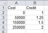
If the cost value we want to find the credit for is in A7, then the VLOOKUP function would look like this:
=VLOOKUP(A7,A2:B5,2)
As you can see, this is a lot less complicated than a formula with multiple IF statements in it. Extending it with new rows is also a lot easier than editing a complex IF formulas to add new conditions.
There are some fish hooks in this approach, however. I recommend you read our lesson on VLOOKUP to find out more.
Regards
David
Nested IFs not "re-calculating" once they've been triggered
Hi ~
So I'm a programmer and understand nested IFs just fine. However, in Excel (and in Open Office), when I use a formula such as this:
=IF(M14<>"";M14/3;IF(G14<>"";G14/2;IF(H14<>"";0;IF(I14<>"";I14/2;IF(J14<>"";J14;0)))))
In a cell, which basically just checks to see if some other cell or cells have information in them, and if they do, uses that information--a number--to perform a calculation for this current cell. The idea is, if I fill in a cell, it'll use it to calculate this dependent cell. Great. Works whenever I fill in the info correctly the first time. However...
When I delete the information in say, M14, or G14, or H14, then this "IF" doesn't re-run. It stays as it was when it first calculated the answer.
Is there a better way, or some way I can tell Excel to re-trigger doing the calculation (re-running the IF statement in this cell) *whenever* I change any of the cells that are contained in the formula above? I'm surprised that Excel doesn't just do this automatically, or that I couldn't find a "re-run all conditionals" menu item, or something similar.
Maybe there is and I just couldn't find it. Or maybe you have a better suggestion for how to accomplish what I'm trying to do (in Excel).
Thanks!
~ Brad
Can't reproduce the problem
Hi Brad
Not sure how to recreate the problem. Can you upload a copy of your spreadsheet?
Excel normally recalculates the entire spreadsheet each time you change a value in a cell. So there are two possibilities:
- You have disabled this automatic recalculation. Pressing F9 will force a recalculation, so check if this makes any difference.
- You are changing values that have no impact on the formula.
Looking at the second point ... if you have a value in M14, then changing the values in the other cells (G14, H14, I14, J14) won't have any impact on the outcome of the formula. This is because the formula stops calculating once it establishes that M14 has a value in it (i.e, M14<>"" is true).
So .... happy to help troubleshoot, but that's my best shot based on the information you've supplied.
David
Tiered Commission Structure!! Help Needed
Hi all
I am having real trouble trying to do this type of commission structure;
£0.00 - £5,000 generated = 0% commission
£5,000 - £10,000 = 15% commission
£10,000 - £15,000 = 17.5% commission
£15,000 - £20,000 = 20% commission
£20,000 - £25,000 = 22.5% commission
£25,000 + = 25% commission
(so, for example, if a person was to generate £16,000 for the business, £5,000 would be non commisionable. The next £5,000 will result in receiving £750.00 (15%). The next £5,000 would be £875.00 commission (17.5%) and the final £1,000 would be @ 20% so another £200. The consultant would earn £750 + £875 + £200 (total of £1,825.00).
How would I put this all into one excel formula? Is there a way to do it so I can input the money a consultant has generated into one cell and the commission is automatically generated into another?
anyone with answer, please
anyone with answer, please share. I want to apply the same logic in calculating kenya PAYE tax
please help
can anyone please give me an Excel formula for this ...thanks
If customers buy one pair of shoes, they receive no discount; two or three pairs of shoes, they receive a discount of 10%; and more than three pairs of shoes, a discount of 15%. In addition, if their purchases are greater than three pairs of shoes and exceed $200, they receive a further discount of 5% (for a total discount of 20%).
If Statements
Hi,
Am trying to determine a Time band value for a cell which depends on days of the week and time within each day that an event occurred.
I need to determine which time range a event occurred based on the day of the week and time of the day. i.e if an event occurred at 7.30am on a Monday it would be in time band 1, 8pm on a Saturday would be in time band 6 etc.
G2 = Day of the week. represented as a number (1-5 for Mon-Fri, 6-7 for Sat-Sun)
H2 = My event time
I2 = Time band I require from 1 to 6.(Or alternatively 3 times of "Other", "Fringe" and "Prime"
Time bands are
Mon-Fri
Other = 0201 - 0759
Fringe = 0800 - 1759
Prime = 1800 - 0200
Sat-Sun
Other = 0201 - 0759
Fringe = 0800 - 1159
Prime = 1200 - 0200
My basic idea of what the formula should be like is
if g2<=5 and H2 is between 0800-1759 then I2=2(or "Fringe")
i then need to run that same statement for each day and time range and that is where i get caught out and lost in "ifs" and "thens" and ()
Any help would be greatly appreciated.
Cheers
Thanks for help
Thanks for helping me out. I was struggling from last 4hrs. Its all done 'because of you'
HELP
F8=IF(G8>0,G8,0, IF(G8>=D8,D8,G8)))
I am using this formula but still getting an error. What I'm trying to do in cell F8 is that if the value is greater than the value in cell G8 then F8=G8, and if G8 is greater than or equal to the value in D8, then F8=D8, else F8=G8.
Question
= IF(IF(OR(D1 = "IN BOOK", D1 = "NOT IN LIBRARY"), J1, MAX(H1, I1)) < 20100000, "2009Below", IF(IF(OR(D1 = "IN BOOK", D1 = "NOT IN LIBRARY"), J1, MAX(H1, I1)) > 20140000, "Jan-Dec2014", IF(IF(OR(D1 = "IN BOOK", D1 = "NOT IN LIBRARY"), J1, MAX(H1, I1)) > 20130000, "Jan-Dec2013", IF(IF(OR(D1 = "IN BOOK", D1 = "NOT IN LIBRARY"), J1, MAX(H1, I1)) > 20120000, "Jan-Dec2012", "Jan-Dec" & VALUE(LEFT(IF(OR(D1 = "IN BOOK", D1 = "NOT IN LIBRARY"), J1, MAX(H1, I1)), 4))))))
This is my existing formula. How can i add-up the year 2015 and 2016 in the logic. If i add up more formula, the uses more levels of nesting is appearing. How can i shorten up this formula? Thanks.
IF function
Thank you very much for that nice tutorial. I am trying to create a formula for a price list.
The price will change depending the number of people :
For instance :
Company between : 10001 and 15000 people will pay 10,000, company between 15001 and 20000 will pay 12 000, do you know what kind of formula I could create ? I would have to use that formula again for 5 different prices, so what I need to do ? Just add AND ?
Thank you very much if you can help me with that!
Sorry If I made some mistakes in English, I am French.
Louis
Kind Regards,
Need help with IF statement
Multiple IF with range values
Hello, thanks for the information. I'm actually struggling with a formula that is not working. I always obtain FALSE.
=IF(C2>0<2000,"95%",IF(C2>2000<5000,"92%",IF(C2>5000<12500,"82%",IF(C2>12500<25000,"70%",IF(C2>25000,"47%")))))
I want assign a percentage according to the value cell C2 possesses.
0-2000: 95%
2000-5000: 92%
5000-12,500: 82%
12,500-25,000: 70%
25,000=: 47%
Would you mind telling me what's wrong with my formula?
IF STATEMENT
=IF(C2>=25000,"47%",IF(C2>=12500,"70%",IF(C2>=5000,"82%",IF(C2>=0,"95%"))))
try the formula above
Can I do this...
I get a set of data each morning, that I copy into the attached Workbook into the Master Sheet. The pivot table data is then refreshed in the first worksheet.
From this pivot table, two summaries are needed - Management Summary and Historical Summary. The Management Summary, I can copy directly from the Pivot Table. It is the same data just in a different format.
The Historical Summary is a bit more complex in that I would like for the sheet to show the make up of people for that day. I would save the work book with a date variance (POB - Day1, POB - Day2, Etc...) On the next day, I would copy a new master table, refresh the pivot table, create a new column (Day 2) then the column look for that particular position, if it doesn't exist under the group it provides a zero (or blank cell), if it does exist, then it returns the total number of people in that position, for that group, for that company.
Should I organize this differently knowing I can change the Pivot table or the Master Table? Can all the different checks on the Pivot table be done in Excel 2013??
RC
Nested IF THEN
Help! I am tyring to write an IF THEN statement for cell C3 that will:
1. Be blank if cell K3 has a date >= a date in B3
2. Be blank if cell K3 is blank
3. Be a 1 if B3 is >= a date in N3 and B3 is <= a date in N4
4. Be blank if B3 is blank
This is what I have so far: =IF(K3 "","",IF(B3<K3,"",IF(B3>=$N$3 AND B3<=$N$4,1,0)))
You can use the AND and OR functions to help achieve this.
Hi JP
Looking at your criteria, I can't see how the logic is constructed. Can you provide more information? For example:
- It looks like B3 has to be non-blank. If it is blank, C3 must also be blank.
- If K3 is blank, C3 must also be blank, even if there is a value in B3.
That part's clear, and you can handle this using an OR function. This formula will return 1 (TRUE) if either B3 or K3 are blank, and 0 if neither of them are blank:
=OR(B3="",K3="")
You could use this OR function as a logical test in the IF formula you are trying to create.
From there:
- If neither B3 nor K3 are blank, but K3>=B3, then C3 must also be blank.
You could write a formula in C3 for this. This formula will return 1 (TRUE) if C3 needs to be blank and 0 if it does not:
=AND(OR(B3="",K3=""),K3>=B3)
At this point, if we have concluded that C3 is not blank so far, then:
- If B3>=N3 AND B3<=N4, C3 should have a 1 in it.
- Otherwise C3 must be blank.
You could write this in a formula as:
=AND(OR(B3="",K3=""),K3>=B3,AND(B3<N3,B3>N4))
The outcome of this formula will, as before, be 1 (TRUE) if C3 should be blank, and 0 if it should not. Let's break it down:
The AND function has 3 arguments in this example. All must be TRUE in order for the AND function to return 1 (TRUE).
- Either B3 or K3 are blank AND
- K3 must be greater than B3 AND
- B3 must be less than N3 AND it must be greater than N4
Notice how I inverted the tests comparing B3 to N3 and N4, so that the final argument will return 1 (TRUE).
That now paves the way to write our IF formula:
=IF(AND(OR(B3="",K3=""),K3>=B3,AND(B3<N3,B4>N4)),"",1)
Hopefully that helps. As you can see, your logical tests lent themselves to a single logical function, constructed from a series of AND and OR functions. This meant that we didn't need to use multiple IF functions in our formula.
Bear in mind that not all scenarios are this straightforward and in many cases you may still need to revert to multiple nested IF functions. The key is to know how to construct the right logical statements for each IF function you need. You can read more about Using logical operators and functions in Excel here.
Regards
David
Thank you all for your
Thank you all for your comments!
I was able to get it do what I wanted. This is what I used: =IF(ISNUMBER(L4)*AND(L4<=D4),"",IF(ISBLANK(D4)*AND(L4="")*AND($C$1>=Sheet1!$B$3),0,IF(ISBLANK(D4),"",IF((D4>=Sheet1!$B$2)*(D4<=Sheet1!$B$3),1,0))))
It may not be elegant, but it is working for me!
JP
Hi JP
Hi JP
Well done - that's great!
You could also use D4="" rather than ISBLANK(D4).
I like the way you've multiplied ISNUMBER(L4) by the result of AND(L4<=D4) - so the result of ISNUMBER(L4) is multiplied by 1 or 0. Not enough people use that trick. One point though - you don't need the AND function since there is only one logical test. Simply put (L4<=D4) to get the same result.
Regards
David
HELP required!!
Hi,
I need an IF Formula for multiple criteria,
for eg - if A1 = A or B or C ( 3 different values, depeding on VLOOKUP result)
B2 should return - 3 different values depending on the results of 3 different IF fuctions - how should i combine them into one single formula?
IF(AND(A1=A,D1*3>6),D*3,6)
IF(AND(A1>B,A1<C,D1*7>6),D*7,6)
IF(AND(A1=C,D1*12>10),D*12,10)
Please help!!
Thank you!!
You can nest these IF functions in a single formula
Hi Jen
I think your problem is that you have a number of outcomes where the outcome is not defined.
For example, what happens in your first formula if A1=A but D1*3 is not greater than 6? It appears that your formula doesn't take account of all possibilities.
It feels to me like you need to test whether A1=A first, and then do other tests. For example::
=IF(A1=A,IF(D1*3>6,D*3,6),value_if_false)
Assuming this formula works the way you want it to, then you could put your next IF formula (comparing A1 to B and C) into this formula in place of the value_if_false.
I'm not 100% sure I follow all the logic of your scenario, so I won't try and construct a whole formula for you, but this is how I'd approach the problem.
Let me know how you get on, and feel free to provide further information to help explain what you're trying to do.
Regards
David
I have been working on
I have been working on created a nested IF for a document I am working on, however I have maneged to make two diffrent IF statemnets that both work but they need to be merged.
The infomation its in relation to is:
J K L N
Start End Cloud
23 01/04/2014 cloud Yes
24 03/03/2014 Overdue
25 22/05/1992 cloud Yes
26 03/03/2014 Overdue
27 01/07/2014 cloud Yes
28 29/06/2014 On Time
29 03/03/2014 10/03/2014 Complete Yes
The two IF's i current have are:
This If statement firstly looks to see if the End column is filled if it is filled then the project is completed and that can be Displayed in column L. Then it takes the start(date) in ciolumn J and adds 10 workdays it then compares this to todays date to see if the project is Overdue or ontime.
=IF(NOT(ISBLANK(K25)),"Complete",IF(WORKDAY(J25,10)<TODAY(),"Overdue","On Time"))
This IF statement looks to see if there is a Yes in the Cloud collumn(N) if there is it then adds 20 working days to the start date then compares that to todays date to see if the project is overdue or on time.
=IF(AND(N26 = "Yes", (WORKDAY(J26,20)<TODAY())),"Overdue", "On Time")
So what I am looking for is these two combined but i always get an error or a emssage saying to many arguments.
What it needs to do is:
1) look to see if their is and end date if there is set column L to complete
2) see if there is a Yes in the cloud collumn if so add 20 workdays to the start date the compare to todays date and set column L to either overdue or on time
3) if the cloud column is empty add 10 workdays to the start date then compare to todays date and set column L to either overdue or ontime.
Any help would be awesome!!!
Worked it out with a lot of
Worked it out with a lot of help from someone but for other people here is the answer:
=IF(NOT(ISBLANK(K24)),"Complete",IF(N24 = "Yes",IF(WORKDAY(J24,20)<TODAY(),"Overdue","On Time"),IF(WORKDAY(J24,10)<TODAY(),"Overdue","On Time")))
Such a simple fix!!
ERROR IN 4 IF
=IF(C8="CHIKKA",400,IF(C8="PILLUKHERA",120,IF(C8="KAITHAL",260,IF(C8=”SAFIDON”,160,IF(C8=”NARWANA”,160,IF(C8=”R.N.K.B”,260,IF(C8=”KALAYAT-SIWAN”,340,IF(C8=”JULANA”,120,IF(C8=”UCHANA”,92,”-”)))))))))
ONLY 3 IF IS WORKING OTHER THEN 3 RESULT SHOWS #NAME? PLEASE HELP ME
Help would be much appreciated
Hi, firstly can I say how helpful the comments on this page have been for me (being a total excel layman...!)
I have been trying for days now to create a nested "IF" formula which does the following:
A1: $dollar amount
A2: date in the past
I need a formula that will calculate, from the date in A2, a daily $ figure being:
1) 7.5% per annum (calculated daily) x A1 for the first 2 years from A2; PLUS
2) 5% per annum (calculated daily) x A1 for the following 3 years.
IE, it is 7.5% per annum for years 1 and 2 and 5% per annum for years 3, 4 and 5 from the start date in A2 - but I need the $ figure calculated daily.
I would be hugely grateful for any assistance anyone could offer - I have been pulling my hair out trying to figure this out!
Thank you very much
Need help with this formula
Please help me work out a formula for this, please note that price changes all the time and depends on number of adult and children input by client. Thank you
easier way of doing this formula
I started down the blue but I didn't even get all the row inputted. is there an easier way of doing this so I can get the totals for each day for each color?
Multiple If's only work for 1st item
I have two problems with this program. First on the first product works in the lookup, second when the link is copied to the box it is no longer a link. Any ideas?
Need help with complex IF formula
Hi -
I have been working on a complex nested IF formula for a while, but cannot seem to get it to work. The goal is to calculate the duration (working days) of a project using start and end dates as input. The formula does not contain any errors, but it returns #VALUE! for every condition. Any help would be greatly appreciated.
Here is the formula (using returns to make it easier to read):
=IF($J$1>P$6,0),
IF($J$2<P$5,0),
IF(AND($J$1<=P$5,$J$2>=P$6),P$7),
IF(AND($J$1<=P$5,$J$2<P$6),(P$6-$J$2)+1),
IF(AND($J$1>P$5,$J$2>P$6),(P$5-$J$1)+1,((P$6-$J$2)+1)-((P$5-$J$1)+1))
Your nested brackets are in the wrong place
Hi Bob
It looks to me like your nested brackets are in the wrong place, i.e the IF functions are not nested at all:
=IF($J$1>P$6,0), IF($J$2<P$5,0),IF(AND($J$1<=P$5,$J$2>=P$6),P$7),IF(AND($J$1<=P$5,$J$2<P$6),(P$6-$J$2)+1),IF(AND($J$1>P$5,$J$2>P$6),(P$5-$J$1)+1,((P$6-$J$2)+1)-((P$5-$J$1)+1))
It should be more like:
=IF($J$1>P$6,0,IF($J$2<P$5,0,IF(AND($J$1 ...etc
I haven't tried to interpret your whole formula, but what you'll hopefully see is that your IF functions are not nested properly - you've actually strung together multiple IF functions in a single formula rather than nesting. That's most likely what's causing your #VALUE error.
Just to reiterate how nesting IF statements together works:
- The IF function accepts three arguments - logical_test, value_if_true, value_if_false.
- Your IF functions have only two - logical_test and value_if_true. You then close the brackets and start a new IF function.
- What you should do in your example is put a comma after the value_if_true and then start the next IF function.
- This second IF function will only be evaluated if the logical_test in the first IF function is evaluated as FALSE. Otherwise it will be ignored.
- You could also use an IF function for the value_if_true argument.
Hopefully that helps. The only other suggestion I would make to help you troubleshoot this formula (once you've nested the IF functions correctly) would be to copy each IF function into a separate cell to test whether it returns the correct results. The problem with large formulas with multiple nested IF functions is figuring out where it's going wrong. This approach of desconstructing the formula into it's different components is one I use often.
Regards
David
It Worked!!
David -
Thanks for your guidance. I applied the changes that you suggested and it worked!!
My IF statements were not nested as you indicated.
Here is what the formula looks like after the changes:
=IF($J$1>O$6,0,
IF($J$2<O$5,0,
IF(AND($J$1<=O$5,$J$2>=O$6),O$7,
IF(AND($J$1<=O$5,$J$2<O$6),O$6-$J$2+1,
IF(AND($J$1>O$5,$J$2>O$6),O$5-$J$1+1,
(O$6-$J$2+1)-(O$5-$J$1+1))))))
Using multiple IF statements in Excel
Thank You! Thank You! Thank You!
IF (AND) statements w/ dates
i am trying to use IF(AND) statement but not getting result I want. Here is my work - I am trying to get an X in the last (complete) column if the date is before, on or after the projected finish date and if the actual finish date is blank then leave a blank in the completion column. I can't seem to get it to X the field if the date in Column E is missing or equal to column D.
C D E
Projected Actual
Start Finish Finish Complete
10/29/2013 7/1/2014 3/31/2014 X
3/1/2014 6/1/2014 7/5/2014 X
8/1/2014 12/31/2014 X
8/1/2014 8/1/2014 8/1/2014
This is the formula I have in Column F IF=(AND(E4<>D4),"X"," "))
What am I missing?
Never mind - was over
Never mind - was over thinking it have figured it out.
I need a IF Formula Containing values of multiple Cells
I Need help to generate a comment of result of multiple students whom results i have entered manually. now i want to generate a statement in remarks like
"Student Name" is Failed (or) Passed in (number of Failed (or) Passed Subjects) out of total subjects i.e. 8. His Marks are (obtained Marks) out of Total Marks.
i Have attached the problem sheet.
Please Help me as soon as possible
Thank you
My Formula was
=IF(AND(L4=0),"B2 Passed in 8 out of 8 Subjects. His marks are K2 out of 160.","B2 Failed in L2 out of 8 Subjects. His marks are K2 out of 160.")
but it is not working as i want it to work.
IF Then statement
I would like to come up with numerical designators for phrases such as no, none, yes, somewhat. For example yes = 2, somewhat = 1, no= 0, none =0? How should my if statement look?
I hope you all die this crap
I hope you all die this crap is worse than ebola
Calculate amount
dear sir
if a1<=1 than value comes to 0, if A1>=1 but <1.6 than value comes 1, if A1 >=1.6 but <1.92 than value comes 1.5
Creating a lookup tool
Hello,
Needing some help. I am trying to make up a lookup tool using post codes. So i want input a post code into cell A1 and then it check the post code database for which price bracket it falls under. At the moment I have =IF(E6=G:G,"National",IF(E6=H:H,"London")) but that doesnt seem to be working. Any suggestions?
Thanks in advance.
Andy
Make the [value_if_true] a formula
I need to calculate the EER (Estimated energy requirement) which has a different formula for each age range.
What I need to be able to do is put the data into the Raw Data Box and for the EER to appear in the designated age range column.
The formula for Women 19-30 years of age is: 354 – (6.91*age [y]) + PA*{ (9.36*weight [kg]) + (726*height [m]) }
This is what I tried: =IF(18<J4<31, (354-6.91*J4+J12*9.36*J11+726*J8), " ") but even when Age = 19 nothing appears.
I am well aware there is a way to generate the values without using the IF function but this is not what I am looking for.
I also tried generating the values in a separate cell (so D9=354-6.91*J4+J12*9.36*J11+726*J8) and then creating the IF statement but I got the same result.
This is what I tried: =IF(18<J4<31, D9, " ").
Pls. help me solve this thing...
Pls.help.me...TY
excel using if and AND functions
im trying to write an expression in excel please help:
"You want to know if a loan is a so- called “subprime” loan and if a loan is “under water.” A
loan is subprime if the borrower’s FICO score was less than or equal to 620 and the loan to
appraised ratio is greater than or equal to 90%"
Need help with multiple function using excel
I've attached an excel table with my query on the function, hope to hear from you soonest possible. thank you
Australian Tax calculator as of 2014
0 – $18,200 Nil
$18,201 – $37,000 19c for each $1 over $18,200
$37,001 – $80,000 $3,572 plus 32.5c for each $1 over $37,000
$80,001 – $180,000 $17,547 plus 37c for each $1 over $80,000
$180,001 and over $54,547 plus 45c for each $1 over $180,000
Where column H and row3 holds yearly income in $
=IF((H3<18200),
0,
IF(AND(H3>18200,H3<37001),
(H3-18200)*0.19,
IF(AND(H3>37000,H3<80001),
3572+(H3-37000)*0.325,
IF(AND(H3>80000,H3<180001),
17547+(H3-80000)*0.37,
54547+(H3-180000)*0.45
)
)
)
)
Hi All,
Hi All,
I want to adjust 5 conditions in one formula .
I have used your trick with this but Iam unable to find solution please help on following conditions:
A 9000-15000 60%
B 15001-25000 55%
C 25001-35000 50%
D 35001-45000 45%
E 45001- ABOVE 40%
where I am using the formula: =IF(C21>9000,C21*0.6,IF(C21>15001,C21*0.55,IF(C21>25001,C21*0.5,IF(C21>35001,C21*0.45,IF(C21>45001,C21*0.4)))))
I want to calculate basic from gross(C21)
on these folowing condition , please help.
--Geeta
check my above calculation,
check my above calculation, http://fiveminutelessons.com/comment/1220#comment-1220
use AND(condition1,condition2) for range.
Ok I also want to add that I
Ok I also want to add that I am using Libre office
Don't know about Libre office
Don't know about Libre office but in MS Excel your solution would be like
=IF(AND(C21>9000,C21<15000),
C21*0.6,
IF(AND(C21>15001,C21<25000),
C21*0.55,
IF(AND(C21>35001,C21<35000),
C21*0.5,
IF(AND(C21>35001,C21<45000),
C21*0.45,
C21*0.40
)
)
)
)
The above formula doesnt
The above formula doesnt matches with my requirement..........
The given formula is helpful
The given formula is helpful till 2nd condition after that (<25001) it is taking 40% :(
please guide me in this...
~Thanks~
Hi Halim,
Hi Halim,
Thank you so much for your guidance...
The formula needs some amendments and this is how it is working:
=IF(AND(C27>=9000,C27<=15000),C27*0.6,IF(AND(C27>15001,C27<=25000), C27*0.55, IF(AND(C27>25001,C27<=35000), C27*0.5, IF(AND(C27>35001,C27<=45000), C27*0.45,C27*0.4) ) ) )
~Thanks Geeta~
Addition of multiple list of values.
I need to set a logic in Data validation option to filter list of values based on some selected values. For example, for value 'X' in a specific cell list of value in another cell will show 'AAA', 'BBB' & 'CCC': for value 'Y' list of value will show 'DDD' 'EEE' & 'FFF' and for value 'Z' list of value will show 'GGG' 'HHH' & 'KKK'.
Using if function for text
Hello, i'm trying to use the if function for text as opposed to numbers, I currently have a giant list of repeating complicated text in Column B that I would like to condense. For example, I tried =IF(B6="A_25-44_Mobile_Audio _:15_Banner_ 300x250_LA","Louisiana",IF(B6="A_25-44_Mobile_Audio _:15_Banner_ 300x250_LA","Louisiana",IF(B6="F_25-44_Mobile_Banner_300x250_DMA","WGU"))) to have excel change the long string to a simpler Louisiana, that I can filter by. When I do this I'm getting a "False", even though I'm 100% certain one of the conditions is correct.
Thanks!
Help please
I am trying to work out a simple "IF" formula but I can’t seem to get it to work? I am quite a novice so i am hoping the solution will be very simple for someone to work out?
Tier 1 >£15000
Tier 2 >£5000 <£14999
Tier 3 >£1 <£4999
Tier 4 £0
I need the formula to just return a 1, 2, 3 or 4 based on a cell reference with a value in it.
If someone could help that will save me huge amounts of time by doing manual updates on my spreadsheet.
I hope this makes sense??
Adam
nested IF statements as OR statements not AND statements
This article is very clear and concise and easy to understand. However, I am hoping that I can do what I'm trying to do. I usually believe if you can think it, you can do it. I'm hoping that's the case here.
Currently I am using the "and" way of nesting IF's:
=IF(C2<=TODAY(), IF(J2="", IF (K2 = "", IF (L2 = "", "Overdue", "OK"))))
However, I need to look at these values separately as "OR" logic.
OK, to oversimplify what I am trying to do is:
I have a Due Date in one field. I first need to check where this date is as it pertains to TODAY(). IF the date is past the due date AND any one of 5 fields are blank (not all 5, but any one of them).
Is there any way that one can do that with Excel (I'm using the latest version as of 1/16/2015)
IF it is considered
multiple if statements
I'm not sure how this can be done but here is my problem::
Multiple cells containing yes/no values and compiling a list of those yes, no values in one cell
Field Header 8 9 10
yes no yes
Desired result in one cell: 8,10
I essentially want to compile a list of all of the different headers in that one row where the value equals yes.
Does anyone have any idea how to do this?
nested if
=IF(B4<400,B4*7%,IF(B4<750,B4*10%,IF(B4<1000,B4*12.5%,B4*16%)))
i think this formula is wrong...arguments must be separated by semicolons ; not commas.
Sum from IF statements
How can I get a sum of the point results in C2:C16? The nested IF worked fine, but I can't get a SUM of that column. I also need to take that sum and divide it by the count in either that column or B2:B16 for the Grade Point Avg.
Must IF statements have numbers?
Hi. I make décor pieces from home and have a costing sheet where I work out my material cost. Different material = different cost, so I want to know if it is possible in excel to type in a word and it automatically works out the cost of that material. Eg: Supawood is ZAR0.006 per CM2. So once I fill the size in, and I choose "supawood" in the material coulomb, I want it to automatically know that for "supawood" it must multiply the area with R0.006. And so forth for all the different material. Is this possible?
Calculating Leave
I need a function that looks to see the number of years an employee has been working for the company together with their salary grade to determine how many days leave they are entitled to:
Years of service are grouped as Less than 3; More than 3; More than 5 and More than 10
Salary grades are from 0-21; 22-28; 29-39 and over 40
eg. Basic leave is 15 days, if you work for the company for more than 3 years and salary grade is 18 you are entitled to 18 days leave etc, i've calculated that there are 15 different results, I would be grateful for any help to come up with the right function.
Help!!
I'm trying to calculate this with an if sum but not having much luck...
If Total Gp <10001 then commission = 10%
If Total Gp >10001 but <15001 then commission = 10% to 10000, 15% on the remainder
If Total Gp >15001 but <25000 then commission = 10% to 10000, 15% on the remainder to 15000 and 20% on the remainder.
so 25000 GP would be 1000 plus 750 plus 2000 so 3750.
I want to have the sum stand alone so I don't have to refer to the table constantly, can anyone help?!
thanks
IF Function if one column is text and the other is numerical
First, great site. I'm so glad I found it! Lots of great lessons in here. My question is:
I have 2 columns:
Status
Vacation Leave
I need to write a formula to show FT = 15 vacation days; PT = 10 vacation days; CN = 5 vacation days; and EX = 0 vacation days.
I've tried everything I can think of. I've been on Youtube looking for help. I've even downloaded a book to see if it would help. I did manage to get FT= vacation days by using this formula:
=IF([@Status]="FT",15,10) -- @Status is the column header
but Excel put 10 in all the other columns (PT, CN, EX). When I try to just use 15,0, I get an error (#name, #value, not enough parentheses, etc.)
When I try to add to the existing formula, I just get errors.
Any help would really be appreciated!
nested IF command
Use this formula:
=IF(<cell name>="FT",15,IF(<cell name>="PT",10,IF(<cell name>="CN",5,0)))
Nested If function Excel 2010
I am trying to add a line to my existing Excel worksheet and have never written a IF statement with more than 7 nested functions (switched from Excel 2003 to Excel 2010). Can someone help with the attached worksheet?
Help Writing a Huge Formula using these lessons
So I have about 3,000 parts that I have to determine the cost for. In order to do this, I have to write a formula that takes the width of the product, the length, and the process used to make it into account. I have all of this data in separate columns, but am having trouble when it comes to wrapping my head around one gigantic equation to cover all the bases.
I also ran into a problem based on the prices only differentiating when the length reaches certain ft. markers. EG: a Construction Grade(CGD) piece that is 2'x4"x10'(Listed in inches in my column, so 120) costs the same as a 2'x4"x9'3" board. So I need an if/then formula that sets certain parameters around data sets, like if less than 120" and greater than 96", and is construction grade, then this is the price...
Let me know if I can help in describing it more clearly. It's taking me forever to pick up the idea of writing huge formulas like this in Excel!
arithmatic operation on nested if values
first of all ,thanks in advance for the people whom create these very nice tutorials.I wanted to do math operation on the results of nested IFs.how could it possible with one formula??? my formula is as this:
=IF(HOUR(D26)>0;HOUR(D26)*45357;IF(MINUTE(D26)>0;MINUTE(D26)*755.95;IF(SECOND(D26)>0;SECOND(D26)*12.6;0)))
---------I wana add a statement to above formula in order to sum the true values , it calculate the first but ignores others!!!! I wanna sum hour+minute+second
If statement
first thank you
that was the best explanation I have had and it was great as a reminder on how to do it and use it . I only needs these once or twice a year and sometimes longer gaps, so it was fantastically well stated
using results from nested IF function in calculation in new cell
Hello,
Your instructions on how to do nested IF functions are very helpful. I would like to use the results from a nested IF function in a new calculation in a new cell. I simply want to multiply the cell with the nested IF calculation by 2. When I enter the command ={select cell with nested IF function}*2, I do not get a numerical result. Alternatively, if there is a way for excel to recognize the number of pay periods in a given month, I would actually multiply by that number, but for the sake of keeping things simple, I can just multiply by 2 as most months only have 2 pay periods.
Thank you!
figured it out
For some reason an error would come up when I tried to calculate a function using the cell with IF function. However, I was able to do the calculation in a cell outside of the table. This has now happened a few times - not sure why, but quick solution is to calculate outside table and then add to the table.
IF functions referencing a cell that has a formula
I have been given a daunting task by my HR manager. We have job grades that have a maximum annual salary. Our bonus structure is based on the employee's job grade and what % of their grade max they are earning.
I thought I had figured out a way to do it, but it's not calculating correctly because the field that I'm referencing (current % of job grade) is a formula. I'm taking their current salary divided by the annual job grade maximum to get their current %.
Is there anyway you could help with this? Thanks!!
Can you clarify what the problem is?
Hi Gillian
I'm not quite sure what the issue is.
In the spreadsheet you attached to your comment, I can see the formula where you are calculating what they would be earning if they were on 100% of their grade. It seems simple to use that in a formula to calculate each person's current salary as a percentage of that 100% total - and I can see that you've already written that formula.
- Is the problem that the results of that formula are inaccurate?
- Or that your calculation of the 100% total for their grade is incorrect?
- Or that you have another formula elsewhere that is using the percentage calculation, and which is not working?
Regards
David
umm help
this is the function I have for an aging chart
=IF(I2<1,"Current",IF(I2>0 AND(i2<31),"1-30",IF(i2>30 AND(i2<61),"31-60",IF(i2>60 AND(i2<91),"61-90",IF(i2>90AND(i2<120),"91-120","120+")))))
what is wrong here
The problem is the way you're using AND
Hi Matt
The problem is that you're using the AND function incorrectly. You can learn how to use the AND function here.
In short, your formula has examples such as this:
I2>0 AND(i2<31)
You should replace this specific example with this:
AND(I2>0,I2<31)
If you do this all four times in your formula it should work, although you also have some logic errors that mean your formula may not return the result you are expecting.
For example, your first logical test says "I2<1". If this is true, the formula will return "Current" and then stop.
However, your second logical test says "I2>0". This overlaps your first test. There are some scenarios where this would be true for both logical tests. I would change the second test to read "I2>=1" to make remove the overlap and make the formula easier to troubleshoot.
I'd also suggest you explore creating a separate table with each of your ranges and the corresponding result for each, and using a VLOOKUP formula instead of multiple IF functions in a formula. This makes the formula a lot simpler and easier to debug. It also makes it easier to change the results messages. You can read about the VLOOKUP function here.
I hope this helps.
Regards
David
Exclude 0
Hi,
thank you for this good explanation. It has worked perfectly for my table I wanted to fix.
Just one question: how can I exclude the 0 in the calculation? In my case the table should count the result from 1 up.
More information please ...
Hi Elisabeth
Could you provide some information about what you are trying to achieve?
Thanks
David
Hi David,
Hi David,
here is my calculation:
=IF(D6<5,1,IF(D6<7,2,IF(D6<9,3,IF(D6<11,4,IF(D6<13,5,IF(D6<15,6,IF(D6<17,7)))))))
the formular should count from the value 1 on and not from 0.
So the first value IF D6<5,1 should show 0 (or even better nothing) if no value is added. I made this formular to calculate automaticly the tables needed for a certain ammount of people, to count the max availability of tables in a restaurant. When I copy the formular to the other rows, it shows me the value 1 even I have not entered any number in D6 (and following rows).
Thanks for your quick answer
Elisabeht
Add another IF statement
Hi Elizabeth
You could solve your problem by adding another IF statement to explicitly exclude 0 values:
=IF(D6=0,"",IF(D6<5,1,IF(D6<7,2,IF(D6<9,3,IF(D6<11,4,IF(D6<13,5,IF(D6<15,6,IF(D6<17,7))))))))
This will check if D6 is 0 or empty (i.e. equivalent to 0) and return an empty value as the result (the cell will have nothing in it). If D6 is not zero, it will carry on and return the correct result.
The other thing that you should be aware of is that if D6 has a value greater than 17, the formula as written will return a result of FALSE. Assuming you want it to return a blank cell, you could modify the formula like this:
=IF(OR(D6=0,D6>=17),"",IF(D6<5,1,IF(D6<7,2,IF(D6<9,3,IF(D6<11,4,IF(D6<13,5,IF(D6<15,6,IF(D6<17,7))))))))
This uses the OR function to check if D6 = 0 OR D6>=17, and returns an empty value in either case.
Also, as I said in an earlier comment, a VLOOKUP function could be a better way to get the same outcome, in a shorter and simpler formula. You can read our VLOOKUP lesson here.
Thank you for your help so
Thank you for your help so far.
Now another question concerning the formular: how can I change the font color of a value.
Following situation:
The restaurant has max. 25 tables. I want the cell automatically change the color of the cell with the value of the tables needed to red if a new entered booking is overbooking the restaurant.
I have entered at the end of the list as total in a cell =SUM(F28+M28) -there are two different times where the guests can eat in the restaurant- and =IF(K31>24,"FULL","AVAILABLE")
stuck!!!
hall hire headcount
from to cost
0 50 300
51 150 450
51 upwards 700
i need to have a formula that if the guests are more than 50 people then then 300 should show up. but i do not know how to do this. please help!!!
stuck!!!
hall hire headcount
from to cost
0 50 300
51 150 450
51 upwards 700
i need to have a formula that if the guests are more than 50 people then then 300 should show up. but i do not know how to do this. please help!!!
Thank you for the informative post, but I can't figure it out
I am trying to find a formula that would work for the following issue
In J7 we would enter 1-6 depending on how many days we are into the work week.
E6 - E11 would have the profit or loss calculated for each of the days of the week Monday - Saturday.
Depending on the number entered it would calculate the profit or loss we had on specific days.
I came up with
IF(J7=1,e6,IF(J7=2,e6:E7,IF(J7=3,e6:E8,IF(J7=4,e6:E9,IF(J7=5,e6:E10,IF(J7=6,e6:E11))))))
but I received the error Err:508
I'm not sure what I am doing wrong.
Help with IF formula needed...in hope!
I am trying to create a formula for a 4x4 grid system with a person putting an 'X' in each row. Depending on which cells have an X in,this will then return a result ("substantial" in this case) based on the 'true value' in the IF formula I have used: =IF(AND(A1="X",B1="X",C1="X",D1="X"),"SUBSTANTIAL","") which works fine for when cells in the formula are 'X'd.
I am struggling to add another IF formula to replicate this but with one cell different (a person might put a X in a different cell (A2 on the grid for example) returning a different value). There are 4 potential outcomes depending on which cells get marked.
I did attempt to include an OR part to the formula i.e. A1 OR B1 AND A2, A3, A4 but this didn't seem to work either.
I'm not sure this makes sense, so hope someone can assist - how do I do this, or indeed, is there an easier way?
Multiple "if" and "and" statements
I need a Solution for multiple if statements and 3 and statements
This is my current formula:
=IF(A2=6102,"1.16",IF(A2=6202,"0.00",IF(A2=6301,"1.12",IF(A2=6401,"1.13",IF(A2=6602,"1.15",IF(A2=6701,"1.13",IF(A2=6801,"1.18",IF(A2=8001,"1.15",IF(A2=8101,"0.00",IF(A2=8201,"0.00",IF(A2=8501,"1.175",IF(A2=8701,"0.00",IF(A2=8901,"0.00")))))))))))))
I need to Add 3 conditions but keep getting an error message
for 6102 there can be 2 outcomes: IF(AND(A2=6102, E2=F2)),"0.00","1.16",IF(and so on....
for 8501 there can be 2 outcomes: IF(AND(A2=8501, E2=F2)),"0.00","1.175",IF(and so on....
for 8001 there can be 2 outcomes: IF(AND(A2=8001, E2=F2)),"0.00","1.15",IF(and so on....
So if both conditions are met then "0.00" , if they are not then "1.15" but all the other non AND statements must also be check as well and the correct match wins.
This was my attempt:
=IF(AND(A2=6102,E2=F2)),"0.00","1.16",IF(A2=6202,"0.00",IF(A2=6301,"1.12",IF(A2=6401,"1.13",IF(A2=6602,"1.15",IF(A2=6701,"1.13",IF(A2=6801,"1.18",IF(AND(A2=8001,E2=F2)),"0.00","1.15",IF(A2=8101,"0.00",IF(A2=8201,"0.00",IF(AND(A2=8501,E2=F2)),"0.00","1.175",IF(A2=8701,"0.00",IF(A2=8901,"0.00")))))))))))))
This is my error message:
"When the first character is an equal (=) or minus (-) sign, Excel thinks it's a formula:"
Should this be an array table or would there be a fix for the formula?
Thank you for your help
Foursome?
Hello,
I have a situation like this:
A (it has possibility to be 0)
B
C
D (it has possibility to be 0)
I need such an IF function that gives me these conditions:
If A=0 and D=0 result= B-C
If A=0 and D<>0 result= B-D
If A<>0 and D=0 result= A-C
If A<>0 and D<>0 result = A-D
Basically what I need is to prioritize A and D, and use them in calculation if they have a value. Otherwise B and D will be used in calculation.
Whatever I tried, I couldn't achieve to separate "true" and "false" conditions to independent true or false conditions. Like this:
I mean like these:
If condition, (if condition true,false) , (if condition true,false)
....................(..THIS IS TRUE........).,.(...THIS IS FALSE.....)
I would be glad if I can get some help!
Thanks in advance,
VLookup / IF / AND - HELP
Column L - What I am trying to do is any readings that are entered into column C if they are lower than the number in column E then it looks at the standard paragraph sheet tab and when I go to create the letter from the create a letter sheet tab that information will populate into the letter. (NOTE: there will be times that the cell shows NA as a number. How do I work around this?)
Column M - Then any readings that are in column D if they are higher than the number in column G it looks at the standard paragraph sheet tab and when I go to create the letter from the create a letter sheet tab that information will populate into the letter. (NOTE: there will be times that the cell shows NA as a number. How do I work around this?)
I can't see to get this to work. Originally had in column L =IF(ISERROR(IF(VLOOKUP('6-12-2015'!$A$16,'Standard Paragraphs'!$A:$D,3,FALSE)<>0,"Yes","")),IF(VLOOKUP('6-12-2015'!$A25,Standard Paragraphs'!$A:$D,3,FALSE)<>0,"Yes",""))
Also tried =(IF(C25<E25,VLOOKUP(a25,'Standard Paragraphs'!$A:$D,3,0),"") but this didn't work.
Also tried IFERROR(IF(AND(($E25)*1>$C25,VLOOKUP($A25,'Standard Paragraphs'!$A:$D,3,FALSE)<>""),"Yes",""),"") When I entered this I either got False or #NA. I don't know if this works at all.
Any help would be great.
NOTE: Need in Excel 2013 Saved in older version to upload
Assistance With A Date Due Spreadsheet
I have a spreadsheet in which it shows me when a certain item is due. My Cell, F2, has the date that certain item has been sent up. Cell G2 already has a formula to reflect that the item will be due to me within 10 business days after F2. H2 has the date the item has been returned. I need K2 to reflect the following:
If H2 is blank, and today is after the date in G2, I need K2 to read overdue, call location. If H2 is filled in with any date, even a date after Today, then I need K2 to read complete.
Any assistance will be great with this.
Thank you.
Nested IF formula
in cell D5
=IF(VLOOKUP(C5,'store1'!$F$4:$F$29,1)=C5,"store1","")&(IF(VLOOKUP(C5,'store2'!$F$4:$F$29,1)=C5,"\store2","")&(IF(VLOOKUP(C5,'store3'!$F$4:$F$29,1)=C5,"\store3","")&(IF(VLOOKUP(C5,'store4'!$F$4:$F$29,1)=C5,"\store4","")&(IF(VLOOKUP(C5,'store5'!$F$4:$F$29,1)=C5,"\store5","")&(IF(VLOOKUP(C5,'store6'!$F$4:$F$29,1)=C5,"\store6","")&(IF(VLOOKUP(C5,'store7'!$F$4:$F$29,1)=C5,"\store7","")&(IF(VLOOKUP(C5,'store8'!$F$4:$F$29,1)=C5,"\store8","")&(IF(VLOOKUP(C5,'store9'!$F$4:$F$29,1)=C5,"\store9","")&(IF(VLOOKUP(C5,'store10'!$F$4:$F$29,1)=C5,"\store10",""))))))))))
I have ten store sheets with working employees name and one "all store employees name" sheet. Sometime few employees work in two store and swipe with store1 to store2 or store3 or other.
What I want is if some employee worked in more then one store then store(mean sheet name) number show in 'all store employees name' sheet.
Example: "all store employees name" c5 to c30 is A to Z alphabet
and f4 to f29 A to Z alphabet in all store
This for formula work but not popper:
A to M show #n/a
Please help and thanks in advance
I apologize for not being word-perfect in English.
If and formula
I have incentive sheet based on two months achieve and three conditions to take percentage of basic amount and when try using if and formula it takes the first condition only and ignore the
Having trouble overriding an IF formula with another option
Hello all,
hoping one of your expertees may be able to help me here i have an IF formula already created that works for tracking if work goes out of target, the target date is entered, and when the completion date is entered is showed a pass or fail. fairly simple. but i want another cell to be able to override this result, so i can have a interim date sent that as long as its also within the alotted time will overide the normal completion date and result in a pass also (even if the completion date goes out of date)
here is my formula
=IF(ISBLANK(B10),"",IF(OR(G10>C10,AND(ISBLANK(G10),TODAY()>C10)),"fail","pass"))
any help would be majorly appreciated and iv also uploaded a sample spreadsheet on here to have a look at too.
kind regards
could someone please have a look at this?
hi can someone please take alook at this as im still struggling with it
I need Help
From the following Table I need to derive a formula which will automatically add up the amount in column F if it has "3A" in Column C. I should get an accumulative total at the end.
3A 6.1 45 0.970
3A 5.5 48 0.995
3B 4.6 48 0.832
3A 4.3 47 0.746
3B 4.6 54 1.053
3A 4.9 50 0.962
3B 4 53 0.882
3B 4.6 49 0.867
3A 4.9 54 1.122
3B 4.3 52 0.913
3A 4.3 52 0.913
3B 5.2 54 1.190
3A 4 52 0.849
3A 4.9 50 0.962
3B 4 52 0.849
3B 6.1 50 1.197
3B 6.1 52 1.295
3B 4.9 51 1.000
3B 4.9 48 0.886
3B 6.1 47 1.058
3A 5.8 52 1.231
if formula
Hi,
Above if formula how to input commission value not to exceeded 200.
Thanks
Tapash
Hi,
Hi,
I'm trying to write a fairly simple formula nesting multiple IFs and SUMs, like so:
=IF(F1="Oct",Sum(L6:U6),IF(F1="Nov", SUM(L6:V6)), IF(F1="Dec", SUM(L6:W6)))
This doesn't work, I get this error: Youve entered too many arguments for this function.
Now, I was under the impression that you can nest up to 64 statements. I'm trying to write this for 12 months, that's 12 IFs and 12 SUMs. Should be in the clear. But it's not even working for three iterations.
Anybody have any ideas here?
Thanks
Lucie
Sorted. Not nested properly.
Sorted. Not nested properly. Duh!!
Please assist help me to
Pleaseassist help me to correct this formula! where is the problem?

The syntax of the formula is incorrect
It looks like the issue is your use of semicolons instead of commas. Try changing to commas and then troubleshoot from there.
Working version of your formula
As a further note to my last comment, the formula as written won't work even if you change the semi-colons for commas.
Here's a working version of the formula:
=IF(C8=1,B36,IF(C8=2,B37,IF(C8=3,B38,IF(C8=4,B39,IF(C8=5,B40,IF(C8=6,B41,IF(C8=7,B42,IF(C8=8,B43,IF(C8=9,B44,"no match")))))))))
Note the inclusion of the "No match" value in the final IF statement for the value_if_false. If you don't include this, the formula will return the value from B44 for any value in C8 that isn't explicitly included in the formula. You can put whatever you like in place of "no match" but you definitely need something there. A couple of ideas for alternatives:
This version of the formula will return 0 if there is no match found for the value in C8. I've removed "no match" but left the comma after B44:
=IF(C8=1,B36,IF(C8=2,B37,IF(C8=3,B38,IF(C8=4,B39,IF(C8=5,B40,IF(C8=6,B41,IF(C8=7,B42,IF(C8=8,B43,IF(C8=9,B44,)))))))))
This formula will return an empty cell if there is no match found for the value in C8. I've change "no match" to "", which means display a blank value:
=IF(C8=1,B36,IF(C8=2,B37,IF(C8=3,B38,IF(C8=4,B39,IF(C8=5,B40,IF(C8=6,B41,IF(C8=7,B42,IF(C8=8,B43,IF(C8=9,B44,"")))))))))
Criteria Based Values
Hello Excel GURU,
Could you suggest a unique solution for below issue where the last column should automatically refill from formula. 10 till column 6 (for GOLD), 13 till column 12 (for DIAMOND), 25 till column 18 (for SILVER) and so on as I have big list for same criteria.waiting for your helpful response. Thanks in advance!
Serial No. GOLD 10
712755 $10.95
713296 $10.10
717453 $9.99
713812 $9.95
716291 $10.10
Serial No. DIAMOND 13
712755 $9.10
713296 $8.85
717453 $8.99
713812 $9.90
716291 $7.99
Serial No. SILVER 25
712755 $8.00
713296 $7.99
717453 $6.99
713812 $7.75
716291 $7.50
herewith the FYA for your reference.
Regards,
Reeya
Need help nesting an IF(OR formula with too many arguments error
Hi all,
I'm attempting to craft a formula that will take the numerical data in cell D5, and, in another cell, calculate if the number in D5 is "OK" or "Ineligible". In this example, I have 185 values that are considered "OK", but I can only add 30 values to the following IF(OR statement before I get a "too many arguments" error. I haven't been able to find a way to Nest an IF(OR statement to allow me to add additional values. Any suggestions?
=IF(ISBLANK(D5),"",IF(OR(D5=1860,D5=1924,D5=2002,D5=2003,D5=2016,D5=2021,D5=2039,D5=2041,D5=2065,D5=2105,D5=2110,D5=2111,D5=2112,D5=2143,D5=2220,D5=2286, D5=2288, D5=2300, D5=2302, D5=2305, D5=2361, D5=2362, D5=2380, D5=2386, D5=2388, D5=2413, D5=2417, D5=2501, D5=2503, D5=2534),"Class OK","Class I/E"))
Thanks in advance,
-Eric
A couple of solutions to consider
There are a couple of ways you could get the result you need based on the information you've supplied.
Option 1 - Multiple IF functions
You should be able to split the OR function across multiple IF statements, This example shows a version of your formula with two IF functions, each using an OR function to evaluate some of the values:
=IF(OR(D5=1860,D5=1924,D5=2002,D5=2003),"Class OK",IF(OR(D5=2016,D5=2021,D5=2039,D5=2041),"Class OK","Class I/E"))
In this example, if D5 matches one of the values in the first OR function, then "Class OK" is returned. If not, then the formula moves on to the next IF function. If D5 matches one of the values in the second OR function, then "Class OK" is returned, otherwise "Class I/E" is returned.
You can read more about using multiple IF statements here.
Option 2 - Use VLOOKUP
My preference would be to use a VLOOKUP function. This allows you to keep the list of 185 values in a separate table, and keep your formula short and easy to troubleshoot:
=IF(ISERROR(VLOOKUP(D5,F7:F12,1,0)),"Class I/E","Class OK")
In this example, the VLOOKUP formula will look in the range F7:F12 for an exact match with the value in D5. If VLOOKUP doesn't find one it will return an error. The ISERROR function will return TRUE if this is the case, so the formula will return "Class I/E". If the ISERROR function is FALSE, then the function will return "Class OK".
Note that the last parameter in the VLOOKUP function is set to 0. This tells VLOOKUP to find exact matches. It means that your list of values can be in any order you like. The alternative value, 1, would look for the nearest value. In this case the list would need to be sorted from smallest to largest.
In this case, the list of numbers will be stored in a range of cells elsewhere in the spreadsheet, You could keep that range in a separate worksheet within the workbook, or even in another workbook altogether if you want. If the list of numbers changes, you'll need to remember to update the formula to ensure the range covers all the cells in the list.
You can read more about how to use VLOOKUP here.
Thanks! I'll try the VLOOKUP
Thanks! I'll try the VLOOKUP option; looks like what I needed!
adding an interim date cell to my formula to overide IF formula
Hello,
hoping one of your expertees may be able to help me here i have an IF formula already created that works for tracking if work goes out of target, the target date is entered, and when the completion date is entered is showed a pass or fail. fairly simple. but i want another cell to be able to override this result, so i can have a interim date sent that as long as its also within the alotted time will overide the normal completion date and result in a pass also (even if the completion date goes out of date and would normally result in a fail)
here is my formula
=IF(ISBLANK(B10),"",IF(OR(G10>C10,AND(ISBLANK(G10),TODAY()>C10)),"fail","pass"))
Obviously the one above works. Iv tried so many alteration of it and just cant get it right with an overiding cell, confused myself that much im not even sure if it needs IF/OR/AND in it :(
any help would be majorly appreciated and iv also uploaded a sample spreadsheet on here to have a look at too.
kind regards
example uploaded for you,.
wasnt sure if i uploaded the example or not so just re uploaded to this reply to make sure
Try this version of your formula
Hi Kye
It seems like a simple problem, but when I looked closely at it, there are actually a lot of different conditions to be considered.
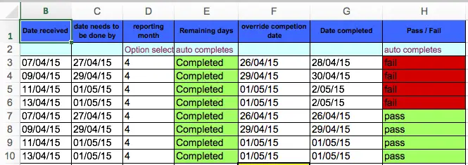
However, from the spreadsheet you supplied, it looks like there are three basic outcomes that the formula in column H should return:
- A blank cell if the value in column B is empty (i.e. the project hasn't been received yet);
- A pass if the project isn't late yet.
- A fail if the project is late.
Here's the formula I wrote to achieve this for row 3. It's a version of your formula, with more conditions within the OR function that you wrote.
=IF(ISBLANK(B3),"",IF(OR(TODAY()<=C3,AND(F3<=C3,NOT(ISBLANK(F3))),AND(NOT(ISBLANK(G3)),G3<=C3)),"Pass","Fail"))
Let's break this down. Notice that there are two IF functions with three possible outcomes:
- The first IF function will return "" (a blank cell), if the Date Received field is empty. If not, the formula proceeds to the next IF function:
- The second IF function will check three scenarios that are considered a Pass. If any one of these are true, the function will return a Pass.
- The due date is today or after today (it's not due yet so it can't be late, regardless of the values entered in F or G);
- The Override date is not empty AND it is not later than the due date;
- The Date Completed date is not empty AND it is not later than the due date.
- If none of the three scenarios above are true, then it should be safe to return a Fail. After all, if the project didn't pass, then it must have failed.
- Bear in mind that there might be some additional Pass scenarios that this formula doesn't consider - these will return a Fail.
- If this is the case, it should be easy to extend the OR function in the second IF function to include more Pass conditions (up to a limit of 32) for the OR function to consider. Remember that with an OR function, you only need one of the conditions to be true for the OR function to return TRUE.
I hope this helps - let me know if you have any further questions.
Regards
David
thank you
thats absolutly brilliant thank you.
One more question
That has all worked really well and im ever grateful for your help. :)
I hope you dont mind me asking this, but is there an easy way to make the "pass" a different colour when being overriden by the interrim date?
Use conditional formatting
Hi Kye
Glad the formula worked - thanks for the feedback.
You can make the Pass a different colour using Conditional Formatting. I can see you've already got a conditional format on the cells to make them either red (fail) or green (pass) - here's what the current Pass conditional formatting rule looks like:
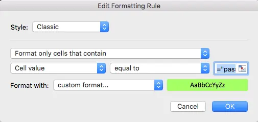
This rule simply looks at the value in the cell to see if it is a Pass or Fail. This rule can stay in place, but you can also add another rule which will use part of the formula in that cell to check if the Pass is due to the override value.
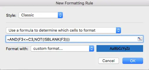
As you can see, I've chosen to "Use a formula to determine which cells to format" rather than your original "Format only cells that contain". I've then taken that part of the original formula that applies to the override column. I've also selected a new colour for the cell.
In order for this to work, you need to select the cells to which you want to apply the rule before starting to create it - this ensures that the rule applies to all relevant cells. Also, note that the forrmula refers to cells in row 3. When you select the cells to apply the rule to, the first row in the selection also needs to be row 3.
Here's what the final rule set for your worksheet should look like with this rule in place. As you'll see, the formula applies to rows H3:H10; the formula refers to cells in row 3. For subsequent cells in the range, Excel will adjust the references in the formula for the row to which the formatting is being applied:
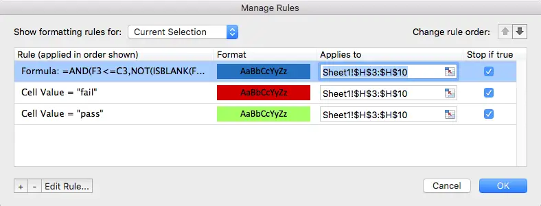
I hope this is what you are looking for. You can learn more about conditional formatting here.
Regards
David
Nested Function Help
Hello, I'm trying to use a nest function for a word to number formula. It works for one formula but I i cant get it working for multiple formulas. i am trying the following =IF(E4="Rare","1",IF,E4="Unlikely,"2")) Unfortunately it wont work, can you please indicate where i'm going wrong?
Thank you
Your directions on using nested if statements was very helpful
thank you.
Is there a way to use if statements by referencing cell colors?
Help me with multiple conditions but some the same, please
Would you please help me how to do if for multiple conditions but some of them will turn out the same value. For example:
States of CA, CO, AR, LA require to do thing on the website
States of AL, AK, IL, require to do thing by using the form
states of DE, DC, IA require to do thing by sending them the letter
some of states require none
If I use IF function will be:
=IF(A2="CA","Website",IF(A2="CO","Website", IF(A2="AR","Website",IF(A2="LA","Website",IF(A2="AL","Form",IF(A2="AK","Form",IF(A2="IL","Form",IF(A2="DE","Letter",IF(A2="DC","Letter",IF(A2="IA","Letter","N/A"))))))))))
Is there any way to reduce that if I to for 50 states and do not need to do write all 50 conditions.
I tried to reduce it
=IF(A2="CO",A2="CA",A2="AR,A2="LA", "Website", IF(A2="AL",A2="AK",A2="IL","Form",IF(A2="DC",A2="DE",A2="IA","Letter","N/A")))
but it didn't work.
Would you please help? Your help is greatly appreciate.
Thanks
Multple Embedded IF Statements or What?
I need help automating summary spreadsheet where another sheet with the selling prices for different products and different selling levels (shown below) would automatically feed the cells in my summary sheet. I need to automate, if the product is product 1,2,3 or 4, at unit sales level X, (shown in the top row of the table below), what is the unit selling price?
ASP UNITS
<15 < 100 100 - 319 320 - 1,599 1,600 - 4,799 4,800 + 9600 +
Prod 1 $96.00 $79.00 $68.00 $60.00 $45.00 $33.00
Prod 2 $63.00 $48.00 $35.00
Prod 3 $106.00 $89.00 $79.00 $72.00 $50.00 $36.00
Prod 4 $65.00 $53.00 $38.00
Multiple IF statements with varying formulas within
Hi,
I am trying to write a formula to calculate a price for a user input length that has varying price points. A long length may have 2-3 calculations to perform. It all looks and makes sense to me put I cannot get it right, if I input anything more than 20 I get a FALSE return. Below is the work sheet with formula. Your input is greatly appreciated.
INPUT BY USER
A3 length 21
LOCKED VARIABLES
A4 min length charge 20
A5 base price 100
A6 ppinch 1.1
A7 ppinch2 1.8
A8 ppinch3 2.04
A9 ppinch limit 49
A10 ppinch limit2 69
Total Price FALSE
FORMULA
=IF(C3<C4,C5,IF(C3>C9,C5+(C6*(C9-C4))+((C3-C9)*C7),IF(C3>C10,C5+(C6*(C6-C4))+((C10-C9)*C7)+((C3-C7)*C8))))
Sales Tax Rate Caluclations
I'm creating a excel sheet on a Sales Order sheet. We have two taxes which can be applied separate. One tax is 5% called GST and the other is 7% called PST. I can do a statement that that applies 1 tax then both together, but I want to keep them separate. Also I can do 1 lline, but if I have multiple lines. I'm having trouble making a statement with the taxes on multiple lines. I've Tried just IF statement, IF SUM, IF OR , IF AND. and no go. Can you suggest to add the tax all together.
one Statement for GST is: =IF(OR(I18="G", I18="GP"), K18*0.05, "")
other statement for PST is: =IF(I18="GP", K18*0.07, "")
Help?
Hi, I am having some trouble with using nested IF functions. I am trying to put an automatic grading system for grades (note: i am not a teacher, just studying for my Excel exam). Here is the function:
=IF(a9<80,C-,IF(A9<85,B-,IF(a9<90,B+,IF(a9<95,A,IF(a9<100,A+,)))
nvm
I fixed, it is all good now. I forgot the " before and after the grading.
Nested If Statement With Multiple Logical Operators
Hello,
I am trying to figure out the code for the following:
If (C2 is not blank AND E2 is not blank) OR (D2 is not blank AND E2 is not blank), report "yes"
Can someone please assist? I am having trouble finding an appropriate example of a working formula.
Need two if statements with 3 conditions
Hi,
Can anyone help me out in this formula?
=if(B2="-","Patient not Found",if(B5>=B31,B5<B33,"Eligible","Not Eligible"))
What about this:
What about this:
0 and 79% of your quota you get 5%
80% to 99% is 10%
and
100% and above you get 15%
But it's not calculated as a whole. Whatever is sold inside of that percentage is paid at that specific commission rate. so for example: If my Quota is $1000 and I sell $1500 I'm going to make 5% for the first 79%, 10% for 80%-99%, and the rest I make 15% on.
HELP
What about this:
What about this:
0 and 79% of your quota you get 5%
80% to 99% is 10%
and
100% and above you get 15%
But it's not calculated as a whole. Whatever is sold inside of that percentage is paid at that specific commission rate. so for example: If my Quota is $1000 and I sell $1500 I'm going to make 5% for the first 79%, 10% for 80%-99%, and the rest I make 15% on.
HELP
Multiply IF
Hi..
I have a formula =IF(AND(P6>16,G6>2,AB6>19,Y6>63),"OVERHEATED OIL","NORMAL"). That was successfully for one condition. But actually the case has more, like :
IF (P6>16,G6>2,AB6>19,Y6>63),"OVERHEATED OIL","NORMAL"
IF (P6>85,G6>13,AB6>1,Y>1), "CORONA IN OIL",NORMAL"
IF (S6>92), "OVERHEATED SELULOSA","NORMAL"
IF(P6>60,G6>5,AB6>2,Y6>2,AE6>30), "ARCHING","NORMAL"
I have tried to combine these IF statement but I always get an error or a message saying to many arguments.
Any give advices/solutions for this case would be awesome!! :D
Thankyou.
Bella
can someone assist?
I am trying to figure out a multiple if statement. I need one cell to produce a formula that will apply for multiple cells and conditions at the same time. for example:
• If any cells equal yellow but NOT red, the result column would be Yellow.
• If all cells equal either green or gray, the result column will be Green.
• If any cells equal red, the result column will be Red.
If command problem
will u please help me to find below condition
if A2 = Dispatched, C2>B2, then D2 = Late,
if A2 = Dispatched, C2<=B2, then D2 = Ontime,
if A2 = Dispatched, C2="", then D2 = Not Done
Help
I am trying to solve a problem with a couple of variables that I could use some help with. I have uploaded the file. I am trying to help sales reps plan on future commissions. I have identified how to write my 1st condition. My sales reps commissions are based on a percent to goal, based on billed monthly revenue * a variable monthly salary amount (cell A29). If the rep is less than a certain percentage, in the uploaded case, 50% then they received no comp. So my first IF statement was written like this =If A26>50%, A26*$A$29, "No Comp"). This handles multiplying anything above 50% to their sales goal times a monthly variable salary (cell A29). The problem is they the reps all have a maximum comp on commissions. In this reps case it is 200% is the max payout percentage, so I don't know how to write the second IF statement which would say if A26 is above 200% the percentage multiplied by cell A29 can only be 200%. Each reps may vary in their maximum monthly percentage. Please assist
MY nested "if" statement is not returning any results.
I am using Excel 2016.
I would like for my nested if to look at column "B2"(contains transaction date) and determine an issue(Winter 2015, Spring 2015, Fall 2015, etc) in column "G2"
My formula is not giving me an error or any results. I tried placing an "=" sign in front of the first "if" and received an error stating "there is a problem with this formula.....
IF(B2<DATEVALUE("05/03/2015"), "Winter 2015", IF(B2<DATEVALUE("07/13/2015"), "Spring 2015", IF(B2<DATEVALUE("10/16/2015"), "Fall 2015", IF(B2<DATEVALUE("04/30/2016),"Winter 2016"))))
Problem with nested "if" statement
I have resolved my own issue. I recreated my nested statement, by building on it...I tested the1st if statement then applied the 2nd, 3rd and 4th. Now its working.
Can you please help
Hi all
I'm trying to write a formula
B1 = ddmmyyyy
B2 = ddmmyyyy
D1 = cost
J1 = proceeds
K1 = profit/loss
In cell N, I want to write a formula that has this meaning:
"If B1-B2 is less than 365 days, then K1. Otherwise K1*50%
=IF(DAY(B1)-DAY(b2)<365,K1,K1*50%)
It only works if number of days is <365 days. "Otherwise" doesn't work.
Please tell me where I've done wrong. Thanks
Too many levels of nesting
Here is my formula:
=IF($B16=0,IF($B15=0,IF($B14=0,IF($B13=0,IF($B12=0,IF($B11=0,IF($B10=0,IF($B9=0,SUM(B7:B8),SUM(B7:B9),SUM(B7:10),SUM(B7:B11),SUM(B7:B12),SUM(B7:B12,B13),SUM(B7:B12,B14),SUM(B7:B12,B15:B16)))
I'm getting a pop-up message:
"The specified formula cannot be entered because it uses more levels of nesting than are allowed in the current file format"
I'm using Excel 2010 Professional
Too many levels of nesting
Problem solved. Compatibility mode was the culprit.
If function
I have a spreadsheet for a property portfolio whereby there is a column for the property reference number - T61-T72. Each of these numbers relates to a separate property for example T61 is Garage 1 T62 is Garage 2 and so on up to Garage 12, I want to have a formula whereby it will fill in the name of the property dependent on the reference. For example a basic IF may be If(I7=T61, Garage 1) however i need to do this for all of the numbers. I hope this makes sense!
Thankyou in advance
Alice
IF Then statement? unsure
I have a table that has $$ amounts and a name associated to those $$'s. On the side of that, I would like a running tally of each persons $$ amounts. I was able to do a single IF statement for 1 line, however I can't seem to figure out how to add multiple lines without creating an error message. For example, if line 4 had $5 in there and named Jose, it would add to Jose's $$ amount....and in line 5 if there was another Chris added, I would like to have them tally up. Can you help?
Multiple IF not working
Looks more complex than is due to going between sheets, however I cannot get it to work! - the same seems to work fine if the Letter (LT, CT, M, D) are replaced with numbers
So the TRUE outcomes are to calculate a sum based on data in two cells, eg. a figure multiplied by another given figure, but where this info comes from is dependant on the Letters typed into a cell - (hence LT, CT Etc.) And the FALSE outcome I need to default to zero if no info is added into the cell asking for the letters. Hope this makes sense!
the formula:
=IF(H19="*LT*",Pricing!F13*'4ZWW 1-2'!I19,IF(H19="*CT*",Pricing!F14*'4ZWW 1-2'!I19,IF(H19="*M*",Pricing!F115*'4ZWW 1-2'!I19,IF(H19="*D*",Pricing!F16*'4ZWW 1-2'!I19,0))))
- Pricing is the sheet the data is coming from
- 4ZWW 1-2 is the sheet the formula is in
Many thanks
nested IFstatement
how to use nested if statement for the following table
00-09 assign 5
10-24 assign 6
25-49 assign 7
50-74 assign 8
75-89 assign 9
90-100 assign 10
I have used the statement =IF(A2 ˃89, “10”, IF(A2 ˃ 74, “9”, IF(A2 ˃ 49, “8”, IF(A2 ˃ 24, “7”, IF(A2 ˃ 9, “6”, “5”)))))
but it shows error message. What is the correct statement?
calculating price per minute
I've been trying to create an if statement that calculates a price/figure from minutes:
example:START STOP Total Time(min) $35 per 1/2 hr
8:00 8:15 15 ? 1.17 per min
10:00 10:45 45 ?
This is what I've tried already: =IF(K9<=30,"$35",IF(K9>30,K9*1.17))
Error in text?
Hi,
In the lesson, shouldn't the statement:
Is commission less than $400? If TRUE, then calculate commission.
be
Are sales less than $400? If TRUE, then calculate commission.
?
Thankyou!
Extremely helpful...
using IF function in calculating with multiple bonus percentage
hi i would like to seek your help with regards on how will i calculate multiple bonuses with set targets.
Please find attached file for your reference.
1% of Actual sales if Target A is achieved
2% of Actual sales if Target B is achieved
3% of Actual sales if Target C is achieved
Hoping for your prompt response.
Thanks
If functions with text and numbers
Im needing to type a commodity in column b. depending on what grain I use (wheat, milo, corn) I need it to come up with the answer from (h-I)*j)*k) and but it in the correct column that has wheat, milo, or corn. Can you please help me! :)
I started with elevator 2 because it has less data to work with
Use this formula in all cells
Hi Kristina
This formula will do what you need:
=IF($B5=D$4,($H5-$I5)*$J5*$K5,"")
To use it, you should paste it into D5 and then copy and paste it down and across. The $ signs (which indicate absolute references) ensure that the formula will work in any cell in columns D-G and any rows within those columns. for example, the formula in G9 looks like this after copying and pasting from D5:
=IF($B12=G$4,($H12-$I12)*$J12*$K12,"")
Only those elements of the formula that didn't have a $ in front of them have changed.
Here's a picture of your spreadsheet so I can illustrate what this formula is doing:
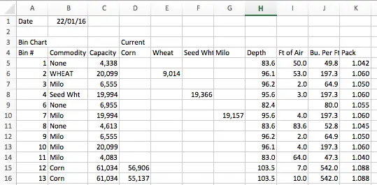
The formula uses a single IF function to check the value in the Commodity column and return the result of the calculation in the appropriate column.
- If the value in column B matches the value in row 4 (whichever column you are in), it will return the calculation.
- If the value in column B doesn't match the value in row 4, it will return an empty cell.
Note that I haven't done anything in the formula to allow for the values in column B where there is no match (i.e the three rows that have None in column B). Here's one way that you might handle that:
=IF(ISERROR(HLOOKUP($B5,$D$4:$G$4,1,0)),"NA",IF($B5=D$4,($H5-$I5)*$J5*$K5,""))
Essentially, this formula checks if the value in column B matches any value in row 4. If it doesn't (as it won't when None has been entered into column B), it returns NA. Otherwise, it completes the calculation of the original formula. This will work regardless of what you type in column B, as long as there is no match in row 4. Note that if you add more commodity columns, you'll need to adjust the HLOOKUP formula. HLOOKUP is a horizontal version of the more commonly used VLOOKUP function;
I have deliberately left an error in the spreadsheet in order to illustrate an important point about this formula. You'll note that rows 3, 9 and 10 don't have a value in the Milo column even though they should.
The reason is simple - the values in column B in those rows don't match the value in G4. When you look more closely, the Milo values in column B have an extra space at the end of the word Milo. This makes them different to the value in G4, so the formula doesn't see them as a match.
I hope this helps. Please reply to this comment if you have any further questions.
Regards
David
multiple IF
dear all, please help me with an IF formula as follows
Start Date 1/04/2015
End Date 31/03/2016
days start date <15 1
days start date >15 0
days end date <15 0
days end date >15 1
Start Date End Date Months covered
20/04/2015 1/01/2017 11
15/02/2014 12
8/11/2015 26/04/2016 5
so I need to calculate the number of months between 01/04/2015 and 31/03/2016, keeping in mind that if the start date is before 15th of the month, that month should be counted as 1. if not it should be counted as 0. if the end date is before 15th of the month, that month should be counted as 0, if not it should be counted as 1.
I don't know whether I should use a count formula with several IF conditions..in the column Months covered is the result I should obtain..
thank youuuuu
best regards
Dana
help
how create excel formulas if:
if the condition is two components is missing
for example:
components
quizzes = 50
project =20
assignment=15
periodical=15
if project and periodical is missing or no values
assignment should be 30% + quizzes = 70%
hope you can help me with my problem
tia
dzeff
Nested If Statement
I need a little help with the following formula. It should be pretty easy, but I am missing something. I worked fine until I added the OR statement to deal with blank fields.
=IF(YEAR(I2)<2014,"Prior to 2014",IF(YEAR(I2)=2014,"2014",IF(YEAR(I2)=2015,"2015",IF(YEAR(I2)=2016,"2016",IF(YEAR(I2)=2017,"2017",IF(OR(I2="",(YEAR(I2)>=2018,”18 And Out",""))))))
Error message when using IF Function
I entered my if formula as:
=IF(K2=A,"$28.17",IF(K2=B,"$17.34",IF(K2=C,"10.84",IF(K2=D,"28.17","$0.00"))))
After hiting enter I get the following error message:
We found a problem with this formula. Try clicking Insert Function on the Formulas tab to fix it, or click Hep for more info on common formula problems.
It will not give me a reason and then asks if I am trying to type a formula which clearly I am. I am not sure where I am going wrong. Any ideas?
Thank you,
Please help
Hope you can help. I am totally out of control for the below calculation.
1) Two Types of Sales Generated by a Sales Rep
a) Treatment - 8000
b) Package / Courses - 8000
Total Sales 16000
2) The Commission Tier
If treatment & Package Sales Total Sum above
a) 0 - 6499.99 - 10%
b) 6500 - 7499.99 - 12%
c) 7500 - 9499.99 - 15%
d) 9500 - 12500 - 18%
Above 12501 x 30%
3) The Above commission tier only apply for Treatment Sales whereby Package sales commission just at flat 8%
My Manual Work
For Treatment Commission
a) 16000-12500=3500 x 30% = 1050
b) 12500-8000=4500 x 18% = 810
For Package/Course Sales @8%
c) 8000 x 8% = 640
Total a - c sum up = 1050+810+640=2500
Multiple conditions
Please help me figure out the right formula using Excel 2013 where the below need to be met:
If Cell A2 contains any of the following texts: C5, R1, R2, or RC1 and there is an error in cell C2, then the outcome will be cell B2*1.05 otherwise if A2 is neither of those AND there is an error in C2 then D2=B2*1.025. If there is no error in C2 irrespective of the value of A2 then the outcome of D2 will be B2.
Column A Column B Column C Column D
C5 323.00 #N/A 339.15
C5 384.00 December 31st 2016 384.00
C1 121.00 #N/A 124.03
C1 145.00 December 31st 2016 145.00
R1 20.00 #N/A 21.00
R2 25.00 #N/A 26.25
RC1 12.00 #N/A 12.60
RC1 12.00 December 31st 2016 12.00
Thanks!!
Help
Im very new at this . I want to be able to select a range of cells from a different sheet that would have the same outcome. For example if anything contained from work sheet 1 appears in a1 of work sheet2 then a2= cat , if not the a2 remains blank.
Pages |
Pleas assist help me to correct this formula
=IF(E1<5999,150,IF(60007999,300,IF(800011999,400,)))
for the table below
Gross Income (Ksh) Monthly Contribution (Ksh)
Less than 5,999 150
6,000 - 7,999 300
8,000 - 11,999 400
12,000 - 14,999 500
15,000 - 19,999 600
20,000 - 24,999 750
25,000 - 29,999 850
30,000 - 49,999 1,000.00
50,000 - 99,999 1,500.00
Over 100,000 2,000.00